Table of Contents
- Definition
- Assumptions
- Types of Logistic Regression
- Formulation
- Analysis Steps
- Binomial Logistic regression
Definition
In statistics, the logistic model (or logit model) is a statistical model that models the log-odds of an event as a linear combination of one or more independent variables. In regression analysis, logistic regression (or logit regression) is estimating the parameters of a logistic model (the coefficients in the linear combination).
Formally, in binary logistic regression there is a single binary dependent variable, coded by an indicator variable, where the two values are labeled “0” and “1”, while the independent variables can each be a binary variable (two classes, coded by an indicator variable) or a continuous variable (any real value). The corresponding probability of the value labeled “1” can vary between 0 (certainly the value “0”) and 1 (certainly the value “1”), hence the labeling; the function that converts log-odds to probability is the logistic function, hence the name. The unit of measurement for the log-odds scale is called a logit, from logistic unit, hence the alternative names.
Binary variables are widely used in statistics to model the probability of a certain class or event taking place, such as the probability of a team winning, of a patient being healthy, etc., and the logistic model has been the most commonly used model for binary regression.
The logistic regression model itself simply models probability of output in terms of input and does not perform statistical classification (it is not a classifier), though it can be used to make a classifier, for instance by choosing a cutoff value and classifying inputs with probability greater than the cutoff as one class, below the cutoff as the other; this is a common way to make a binary classifier.
Logistic regression predicts the output of a categorical dependent variable. Therefore the outcome must be a categorical or discrete value. It can be either Yes or No, 0 or 1, true or False, etc. but instead of giving the exact value as 0 and 1, it gives the probabilistic values which lie between 0 and 1.
Logistic regression is a supervised machine learning algorithm widely used for binary classification tasks, such as identifying whether an email is spam or not and diagnosing diseases by assessing the presence or absence of specific conditions based on patient test results.
Logistic regression uses the concept of predictive modeling as regression; therefore, it is called logistic regression, but is used to classify samples; Therefore, it falls under the classification algorithm.
Assumptions
Given below are the basic assumptions that a logistic regression model makes regarding a dataset on which it is applied:
- Independent observations: Logistic Regression algorithm requires little or no multicollinearity among the independent variables. It means that the independent variables should not be too highly correlated with each other.
- Binary dependent variables: Logistic Regression model requires the dependent variable to be binary, multinomial or ordinal.
- Linearity relationship between independent variables and log odds: Logistic Regression model assumes linearity of independent variables and log odds.
- No outliers: There should be no outliers in the dataset.
- Large sample size: The success of Logistic Regression model depends on the sample sizes. Typically, it requires a large sample size to achieve the high accuracy.
Types of Logistic Regression
On the basis of the categories, Logistic Regression can be classified into three types:
- Binomial: the dependent variable has two possible categories, such as 0 or 1, good or bad, true or false, etc.
- Multinomial: the dependent variable has three or more categories which are not in any particular order. , such as “notebook”, “textbook”, or “reference”
- Ordinal: the dependent variable has three or more ordinal categories, such as “bad”, “normal”, or “good”.
Formulation
Logistic regression is a statistical method used for binary classification tasks in machine learning. It’s a type of regression analysis where the dependent variable is categorical (usually binary) rather than continuous. Formulating logistic regression involves modeling the probability that a given input belongs to a particular class.
Here is a list of the key components:
- Sigmoid Function (Logistic Function): Logistic regression uses the logistic function (or sigmoid function) to map input features to a value between 0 and 1. The sigmoid function is defined as:𝜎(𝑧)=11+𝑒−𝑧σ(z)=1+e−z1Where 𝑧z is the linear combination of input features and their corresponding weights.
- Linear Combination of Features: Similar to linear regression, logistic regression also involves the linear combination of input features and their corresponding weights. However, instead of directly predicting the output, this linear combination is passed through the sigmoid function to obtain the probability.
- Loss Function: Logistic regression typically uses the cross-entropy loss function (also known as log loss) to measure the difference between predicted probabilities and actual class labels.
- Gradient Descent: To optimize the weights of the logistic regression model, gradient descent or its variants are often employed to minimize the loss function.
The formulation of logistic regression involves finding the optimal weights that minimize the difference between predicted probabilities and actual class labels, thus making it a powerful tool for binary classification tasks in machine learning.
# show logistic function(sigmoid function) and its derivative(This is not project part)
import matplotlib.pyplot as plt
import numpy as np
z = np.linspace(-50, 50, 101)
s = np.ones(len(z))/(1 + np.exp(-z))
plt.plot(z, np.ones(len(z))/(1 + np.exp(-z)), "-b", label="Sigmoid")
plt.plot(z, s*(1-s), "--r", label="Derivative of sigmoid")
plt.title("Logistic function")
plt.xlabel("z")
plt.legend(loc="upper left")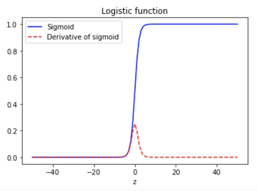
Analysis Steps
Here are the key steps to understand a our model:
- Data Collection: Gather the dataset containing the relevant information we want to model.
- Data Visualization and Data preprocessing:
- Data cleaning: Check for missing values and outliers.Handle them appropriately by imputing missing data or removing outliers
- Feature Selection/Engineering: Determine which independent variable are relevant for our model. we might need to transform or engineer features to make them suitable for regresion
- Assumption Check: If the given assumptions is not satisfied, we may need to apply transformations or consider different modeling techniques.
- Split Data: Divide our dataset into a training set and testing set. The training set is used to train the model and the testing set is sued to evaluate its preformance.
There are several methods for spliting datasets for machine learning and data analysis, Each method serves different purpose and has its advantages and disadvantages. Here are some comon dataset splitting methods along with step by step explanations for each:- Train-test Split(Holdout Method) – purpose to create two seperate sets, one for training and one for testing the mocel
Steps:- Randomly shuffle the dataset to ensure teh data is well distributed.
- Split the data into two parts, typically with a ratio like 70-30 or 80-20, where one part is for training and the other for testing
- Train our machine learning model on the training set
- Evaluate the model performance on the test set
K-Fold Cross Validation: Purpose to assess the model’s performance by training and testing it on different subsets of the data. steps: A. Divide the dataset into K equal sized folds B. For each fold(1 to K) treat it as a test set and the remaining K-1 folds as the training set. C. Train and evaluate the model on each of the K iterations. D. Calculate performance metrics(accuracy) by averaging the results from all iterations.
startified Sampling: purpose to ensure that the proportion of different classes in the dataset is maintained in teh train and test sets steps: A. Identify the target variable B. Stratify the data by the target variable to create representative subsets. C. perform a train_test split on these stratified subsets to maintain class balance in both sets
Time series split: purpose for time series data where the order of data oints matter steps A. sort the dataset based on the time or date variable B. Divide the data into training and testing sets such that the training set consists of past data and the testing set contains future data. - Leave one out cross validation – Purpose to leave out a single data point as the test set in each iteration. Steps: For each data point in the dataset, create a training set with all other data points. Train and test the model for each data point separately. Calculate the performance metrics based on the predictions from each iteration.
Group k-fold cross validation:purpose to accouont for groups or slusters in the data
Steps:- Randomly sample data points with replacement to create multiple bootstrap samples.
- Train and evaluate the model on each bootstrap sample.
- Calculate performance metrics based on the results of each sample.
- Train-test Split(Holdout Method) – purpose to create two seperate sets, one for training and one for testing the mocel
- Model Building:
- Choose the model: select either 3 types of models according to the values of dependent variable: binomial or multinomial, ordinal
- Fit the model: use the training data to estimate the coefficients that maximizes the likelihood of observing the data given
- Model Evaluation:
- Assess Model fit: Use appropiate metrics like acuracy, precision, recall, f1 Score, AUC-ROC or AUC-PR to evaluate how well our model fits the training data.

- Area Under the Receiver Operating Characteristic Curve (AUC-ROC): The ROC curve plots the true positive rate against the false positive rate at various thresholds. AUC-ROC measures the area under this curve, providing an aggregate measure of a model’s performance across different classification thresholds.
- Area Under the Precision-Recall Curve (AUC-PR): Similar to AUC-ROC, AUC-PR measures the area under the precision-recall curve, providing a summary of a model’s performance across different precision-recall trade-offs.
Test the model: Apply the model to the testing set to assess its predictive accuracy on unseen data
Binomial Logistic Regression
Problem Statement
We are going to predict diabetes based on several factors.
Data
CSV file contains all the information. Here are the names of variables.
- Pregnancies
- Glucose
- BloodPressure
- SkinThickness
- Insulin
- BMI
- DiabetesPedigreeFunction
- Age
- Outcome
Import Necessary Libraries
NumPy is a Python library used for working with arrays. It also has functions for working in domain of linear algebra, fourier transform, and matrices. NumPy can be used to perform a wide variety of mathematical operations on arrays. It adds powerful data structures to Python that guarantee efficient calculations with arrays and matrices and it supplies an enormous library of high-level mathematical functions that operate on these arrays and matrices.
Pandas is a Python library used for working with data sets. It has functions for analyzing, cleaning, exploring, and manipulating data. Pandas is a fast, powerful, flexible and easy to use open source data analysis and manipulation tool, built on top of the Python programming language.
Matplotlib is a comprehensive library for creating static, animated, and interactive visualizations in Python. Matplotlib makes easy things easy and hard things possible. Create publication quality plots. Make interactive figures that can zoom, pan, update. Customize visual style and layout.
Seaborn is a Python data visualization library based on matplotlib. It provides a high-level interface for drawing attractive and informative statistical graphics. It builds on top of matplotlib and integrates closely with pandas data structures. Seaborn helps we explore and understand our data.
Scikit-learn is probably the most useful library for machine learning in Python. The sklearn library contains a lot of efficient tools for machine learning and statistical modeling including classification, regression, clustering and dimensionality reduction.
# Supress Warnings
import warnings
warnings.filterwarnings('ignore')

# import the numpy and pandas packages
import numpy as np
import pandas as pd

# to visualize data
import matplotlib.pyplot as plt
import seaborn as sns

# to split arrays or matrices into random train and test subsets
from sklearn.model_selection import train_test_split

# to import logistic regression model
from sklearn.linear_model import LogisticRegression

from sklearn.metrics import accuracy_score
from sklearn.preprocessing import StandardScaler
Data Collection
# data source
url = "./logisticRegression_diabetes.csv"
# reading data
df = pd.read_csv(url)
df.head(10)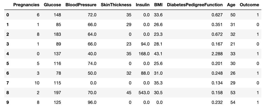
row_cnt0 = df.shape[0]
print("The number of rows : %d." % row_cnt0)
The number of rows : 772.
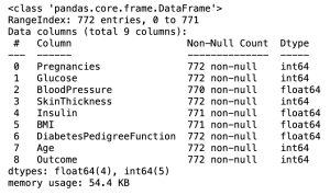
The row count is 772 and the number of variables is 9.
# data information
df.info()
In the Pandas library, the info() method prints summary information about the DataFrame.
Data Processing
- Removing null values
- Removing the duplicated values
- Removing outlier: In the only case that a variable has numerical values not string, we can think about outlier. In the case of string variable, it is neccesary to convert the string values into labels.
- Removing the unneccesary variables
# Checking Null values
df.isnull().sum()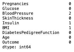
There are NULL values in columns: BloodPressure, Insulin, BMI.
# Removing Null values
df = df.dropna(how='any',axis=0)
row_cnt1 = df.shape[0]
print("The number of rows deleted : %d" % (row_cnt0 - row_cnt1))
The number of rows deleted : 4
df.isnull().sum()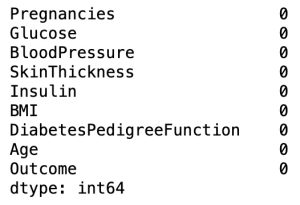
# Checking for the presence of duplicate values. If there exists, we have to remove the rows.
df.duplicated().sum()
There are no the duplicate values.
# Outlier Analysis for Pregnancies
fig, axs = plt.subplots(1, figsize = (6,2))
sns.boxplot(df['Pregnancies'], ax = axs)
plt.tight_layout()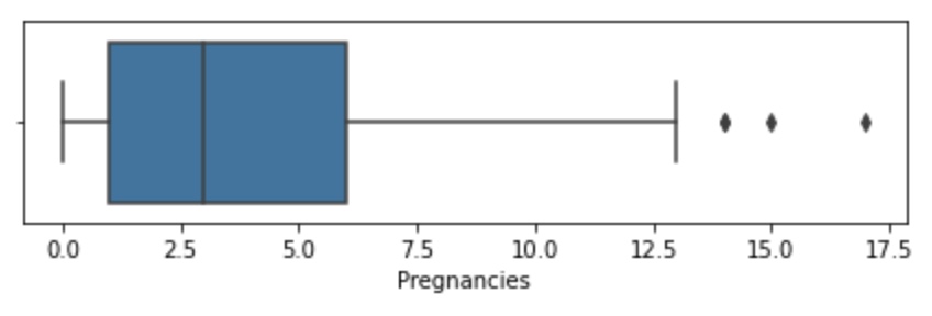
There are considerable outliers in the data. Thus, we can remove larger values of pregnancies than 16.
df = df[df['Pregnancies']<=16]
print("The number of rows deleted : %d" % (row_cnt1 - df.shape[0]))
The number of rows deleted : 1
There are 9 columns and 767 rows in our data set.
Feature Selection
Univariate Analysis: Diabetes (Target Variable)
# we can see each relationship between variables.
sns.pairplot(df)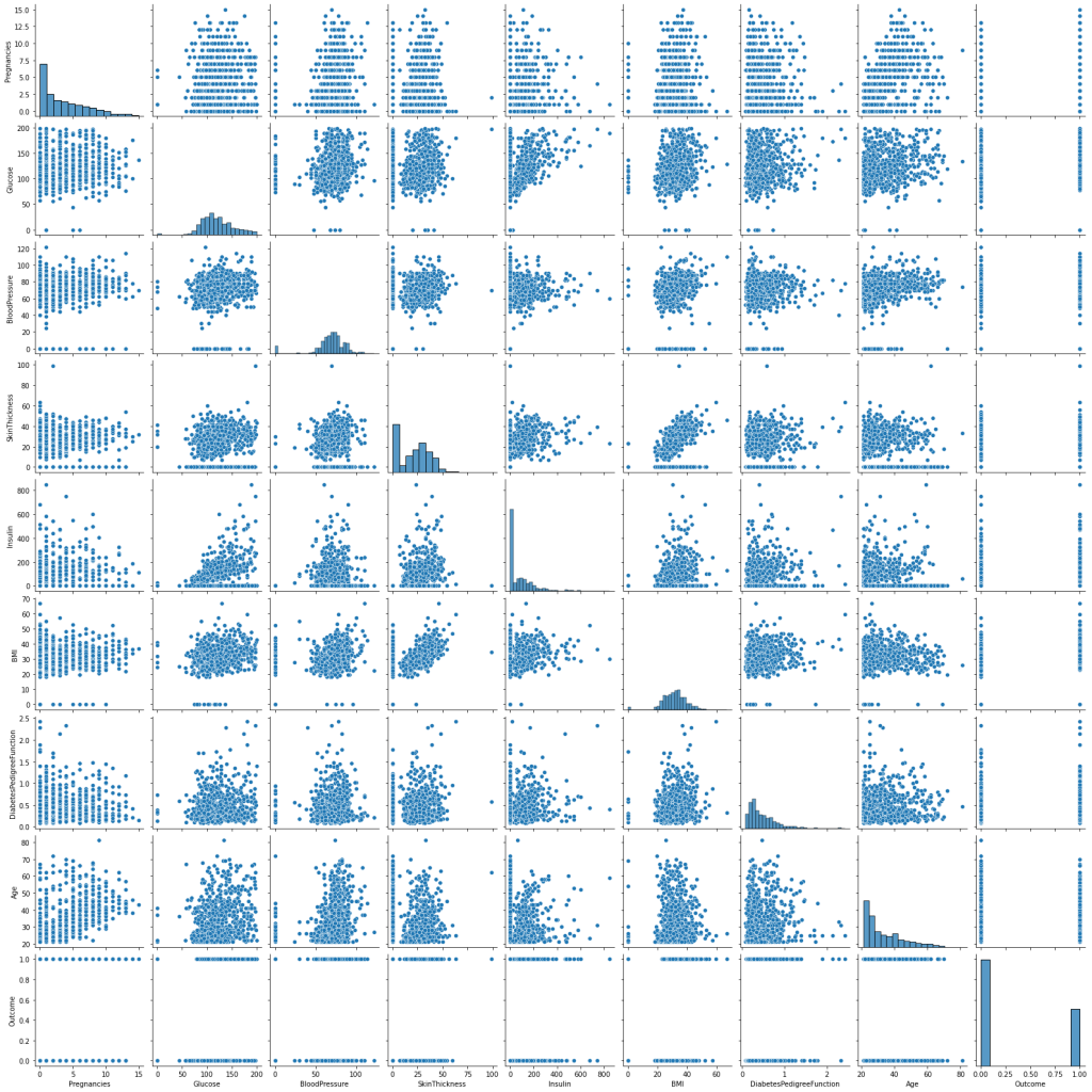
# Evaluating correlation of variables to prevent overfitting
plt.figure()
sns.heatmap(df.corr(),annot=True, cmap='CMRmap_r')
plt.show()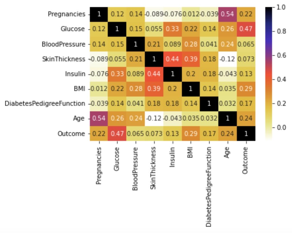
From the above correlation, there are no strong correlations between independent variables. Therefore, we use all independent variables.
Train-Test Split
It is usually a good practice to keep 70% of the data in train dataset and the rest 30% in test dataset.
# Independent variables and dependent variable
X = df.drop('Outcome', axis=1)
y = df['Outcome']

# Standardizing input(independent) variables
scalar = StandardScaler()
scaled_X = scalar.fit_transform(X)

# data split
X_train, X_test, y_train, y_test = train_test_split(scaled_X, y, train_size = 0.7, test_size = 0.3, random_state = 50)
X_train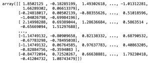
y_train.head()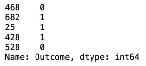
Building Logistic Regression Model
# Creating model
model=LogisticRegression(C=100, solver='liblinear')
# Fitting train data
model.fit(X_train, y_train)
# Predicting based on train data
y_pred_train = model.predict(X_train)
y_prob_train = model.predict_proba(X_train)
y_prob_train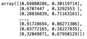
# Predicting based on test data
y_pred_test = model.predict(X_test)
y_prob_test = model.predict_proba(X_test)
y_prob_test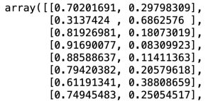
Model Evaluation
Comparison of accuracies for train and test datasets
print('accuracy score for train dataset: %f.3' % accuracy_score(y_train, y_pred_train))
print('accuracy score for test dataset: %f.3' % accuracy_score(y_test, y_pred_test))
accuracy score for train dataset: 0.785448.3
accuracy score for test dataset: 0.740260.3
The accuracies are similar and thus, there is no overfitting.
We cannot say that our model is very good based on the above accuracy. We must compare it with the null accuracy. Null accuracy is the accuracy that could be achieved by always predicting the most frequent class.
y_test.value_counts()
# Null accuracy
accuracy_null = 146 / (146 + 85)
accuracy_null
accuracy null: 0.6320346320346321
Accuracy for the test data is higher than null accuracy and we can use the logistic model in prediction.
Confusion Matrix
A confusion matrix is a performance evaluation tool in machine learning, representing the accuracy of a classification model. It displays the number of true positives, true negatives, false positives, and false negatives.
- True positives (TP) occur when the model accurately predicts a positive data point.
- True negatives (TN) occur when the model accurately predicts a negative data point.
- False positives (FP) occur when the model predicts a positive data point incorrectly.
- False negatives (FN) occur when the model mispredicts a negative data point.
# confusion matrix
from sklearn.metrics import confusion_matrix

confusion_m = confusion_matrix(y_test, y_pred_test)sns.heatmap(confusion_m, annot=True, fmt='d', cmap='CMRmap_r')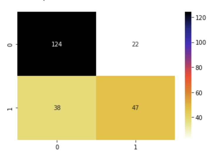
Classification Report
from sklearn.metrics import classification_report

print(classification_report(y_test, y_pred_test))
ROC Curve
from sklearn.metrics import roc_curve

fpr, tpr, thresholds = roc_curve(y_test, y_pred_test, pos_label = 1)
plt.figure(figsize=(6,4))
plt.plot(fpr, tpr, linewidth=2)
plt.plot([0,1], [0,1], 'r--' )
plt.rcParams['font.size'] = 12
plt.title('ROC curve for classifier')
plt.xlabel('False Positive Rate')
plt.ylabel('True Positive Rate')
plt.show()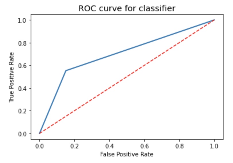

Leave a Reply