Decision Tree

Table of Contents

Definition
Assumptions
Types of Decision Tree
Formulation
Analysis Steps
Classification problem by Decision Tree

Definition

A decision tree is a decision support hierarchical model that uses a tree-like model of decisions and their possible consequences, including chance event outcomes, resource costs, and utility. It is one way to display an algorithm that only contains conditional control statements. A decision tree is a flowchart-like structure in which each internal node represents a “test” on an attribute (e.g. whether a coin flip comes up heads or tails), each branch represents the outcome of the test, and each leaf node represents a class label (decision taken after computing all attributes). The paths from root to leaf represent classification rules. In decision analysis, a decision tree and the closely related influence diagram are used as a visual and analytical decision support tool, where the expected values (or expected utility) of competing alternatives are calculated.

Decision tree learning is a supervised learning approach used in statistics, data mining and machine learning. In this formalism, a classification or regression decision tree is used as a predictive model to draw conclusions about a set of observations.

A tree is built by splitting the source set, constituting the root node of the tree, into subsets — which constitute the successor children. The splitting is based on a set of splitting rules based on classification features. This process is repeated on each derived subset in a recursive manner called recursive partitioning. The recursion is completed when the subset at a node has all the same values of the target variable, or when splitting no longer adds value to the predictions.

Assumptions

There are the assumptions below.

In the beginning, the whole training set is considered as the root.
Feature values are preferred to be categorical. If the values are continuous then they are discretized prior to building the model.
Records are distributed recursively on the basis of attribute values.
Order to placing attributes as root or internal node of the tree is done by using some statistical approach.

Types of Decision Tree

The types of decision trees are based on the values of dependent(target) variable we have.

It can be of two types:

Classification trees: has a categorical target variable. Tree models where the target variable can take a discrete set of values are called classification trees; in these tree structures, leaves represent class labels and branches represent conjunctions of features that lead to those class labels.
Regression trees: has a continuous target variable. Decision trees where the target variable can take continuous values (typically real numbers) are called regression trees. More generally, the concept of regression tree can be extended to any kind of object equipped with pairwise dissimilarities such as categorical sequences.

Decision Tree Algorithms

The decision of making strategic splits heavily affects a tree’s accuracy. The decision criteria are different for classification and regression trees.

Decision trees use multiple algorithms to decide to split a node into two or more sub-nodes. The creation of sub-nodes increases the homogeneity of resultant sub-nodes. In other words, we can say that the purity of the node increases with respect to the target variable. The decision tree splits the nodes on all available variables and then selects the split which results in most homogeneous sub-nodes.

The algorithm selection is also based on the type of target variables. Let us look at some algorithms used in Decision Trees:

ID3: Iterative Dichotomiser 3
C4.5: successor of ID3
CART: Classification And Regression Tree
__CHAID:__Chi-square automatic interaction detection). Performs multi-level splits when computing classification trees
MARS: extends decision trees to handle numerical data better

The ID3 algorithm builds decision trees using a top-down greedy search approach through the space of possible branches with no backtracking. A greedy algorithm, as the name suggests, always makes the choice that seems to be the best at that moment.

Here, we will show the steps of ID3 algorithm.

It begins with the original set S as the root node.
On each iteration of the algorithm, it iterates through the very unused attribute of the set S and calculates Entropy(H) and Information gain(IG) of this attribute.
It then selects the attribute which has the smallest Entropy or Largest Information gain.
The set S is then split by the selected attribute to produce a subset of the data.
The algorithm continues to recur on each subset, considering only attributes never selected before.

Formulation

Decision tree formulation in machine learning involves creating a tree-like model of decisions. It’s a supervised learning algorithm that can be used for both classification and regression tasks. Here’s a basic rundown of the formulation:

Tree Structure: A decision tree consists of nodes, branches, and leaves. Each internal node represents a feature or attribute, each branch represents a decision rule based on that feature, and each leaf node represents the outcome or decision.
Splitting Criteria: At each internal node, the decision tree algorithm selects the best feature to split the data based on certain criteria. The commonly used criteria include Gini impurity for classification tasks and mean squared error for regression tasks.
Recursive Partitioning: The dataset is recursively split into subsets based on the selected feature and its possible values. This process continues until a stopping criterion is met, such as reaching a maximum tree depth, having nodes with minimum samples, or when no further improvement in impurity or error is possible.
Leaf Node Assignment: Once the splitting process is complete, each leaf node is assigned a class label (in classification) or a predicted value (in regression) based on the majority class or average value of the instances in that node.
Pruning (Optional): After building the tree, pruning techniques may be applied to avoid overfitting. Pruning involves removing parts of the tree that do not provide significant predictive power on unseen data.

Decision trees are intuitive, easy to interpret, and can handle both numerical and categorical data. However, they can be prone to overfitting, especially when the tree grows too deep or when the dataset is noisy. Techniques like pruning, setting maximum tree depth, or using ensemble methods like random forests can help mitigate these issues.

Analysis Steps

Here are the key steps to understand a our model:

Data Collection: Gather the dataset containing the relevant information we want to model.
Data Visualization and Data preprocessing:
- Data cleaning: Check for missing values and outliers.Handle them appropriately by imputing missing data or removing outliers
- Feature Selection/Engineering: Determine which independent variable are relevant for our model. we might need to transform or engineer features to make them suitable for regresion
Assumption Check: If the given assumptions is not satisfied, we may need to apply transformations or consider different modeling techniques.
Split Data: Divide our dataset into a training set and testing set. The training set is used to train the model and the testing set is sued to evaluate its preformance.
There are several methods for spliting datasets for machine learning and data analysis, Each method serves different purpose and has its advantages and disadvantages. Here are some comon dataset splitting methods along with step by step explanations for each:
1. Train-test Split(Holdout Method) – purpose to create two seperate sets, one for training and one for testing the mocel
  Steps:
  - Randomly shuffle the dataset to ensure teh data is well distributed.
  - Split the data into two parts, typically with a ratio like 70-30 or 80-20, where one part is for training and the other for testing
  - Train our machine learning model on the training set
  - Evaluate the model performance on the test set
  K-Fold Cross Validation: Purpose to assess the model’s performance by training and testing it on different subsets of the data. steps: A. Divide the dataset into K equal sized folds B. For each fold(1 to K) treat it as a test set and the remaining K-1 folds as the training set. C. Train and evaluate the model on each of the K iterations. D. Calculate performance metrics(accuracy) by averaging the results from all iterations.
  
  startified Sampling: purpose to ensure that the proportion of different classes in the dataset is maintained in teh train and test sets steps: A. Identify the target variable B. Stratify the data by the target variable to create representative subsets. C. perform a train_test split on these stratified subsets to maintain class balance in both sets
  
  Time series split: purpose for time series data where the order of data oints matter steps A. sort the dataset based on the time or date variable B. Divide the data into training and testing sets such that the training set consists of past data and the testing set contains future data.
2. Leave one out cross validation – Purpose to leave out a single data point as the test set in each iteration. Steps: For each data point in the dataset, create a training set with all other data points. Train and test the model for each data point separately. Calculate the performance metrics based on the predictions from each iteration.
  Group k-fold cross validation:purpose to accouont for groups or slusters in the data
  Steps:
  - Randomly sample data points with replacement to create multiple bootstrap samples.
  - Train and evaluate the model on each bootstrap sample.
  - Calculate performance metrics based on the results of each sample.
The choice of dataset splitting method depends on the specific problem, and teh goal of our analysis. its important to select an appropriate method to ensure reliable model evaluation and generalization
Model Building:
1. Choose the model: select either 3 types of models according to the values of dependent variable: binomial or multinomial, ordinal
2. Fit the model: use the training data to estimate the coefficients that maximizes the likelihood of observing the data given
Model Evaluation:
If our problem is Regression problem, use appropiate metrics like Mean Squared Error(MSE), Root Mean Squared Error(RMSE) or R-squared to evaluate how well our model fits.
If our problem is Classification problem, use appropiate metrics like acuracy, precision, recall, f1 Score, AUC-ROC or AUC-PR to evaluate how well our model fits.

Classification problem by Decision Tree

Problem Statement

There is a dataset including the default of credit card of clients and other information. Here, we are going to predict if clients use their default credit cards or not.

Data

CSV file contains all the information. Here are the names of variables.

LIMIT_BAL: Amount of the given credit (NT dollar). It includes both the individual consumer credit and his/her family (supplementary) credit.
SEX: Gender (1 = male; 2 = female).
EDUCATION: Education (1 = graduate school; 2 = university; 3 = high school; 4 = others).
MARRIAGE: Marital status (1 = married; 2 = single; 3 = others).
AGE: Age (year).
PAY_1: the repayment status in September, 2005. The measurement scale for the repayment status is: -1 = pay duly; 1 = payment delay for one month; 2 = payment delay for two months; . . .; 8 = payment delay for eight months; 9 = payment delay for nine months and above.
PAY_2: the repayment status in August, 2005. The measurement scale for the repayment status is: -1 = pay duly; 1 = payment delay for one month; 2 = payment delay for two months; . . .; 8 = payment delay for eight months; 9 = payment delay for nine months and above.
PAY_3: the repayment status in July, 2005. The measurement scale for the repayment status is: -1 = pay duly; 1 = payment delay for one month; 2 = payment delay for two months; . . .; 8 = payment delay for eight months; 9 = payment delay for nine months and above.
PAY_4: the repayment status in June, 2005. The measurement scale for the repayment status is: -1 = pay duly; 1 = payment delay for one month; 2 = payment delay for two months; . . .; 8 = payment delay for eight months; 9 = payment delay for nine months and above.
PAY_5: the repayment status in May, 2005. The measurement scale for the repayment status is: -1 = pay duly; 1 = payment delay for one month; 2 = payment delay for two months; . . .; 8 = payment delay for eight months; 9 = payment delay for nine months and above.
PAY_6: the repayment status in April, 2005. The measurement scale for the repayment status is: -1 = pay duly; 1 = payment delay for one month; 2 = payment delay for two months; . . .; 8 = payment delay for eight months; 9 = payment delay for nine months and above.
BILL_AMT1: Amount of bill statement (NT dollar). Amount of bill statement in September, 2005.
BILL_AMT2: Amount of bill statement (NT dollar). Amount of bill statement in August, 2005.
BILL_AMT3: Amount of bill statement (NT dollar). Amount of bill statement in July, 2005.
BILL_AMT4: Amount of bill statement (NT dollar). Amount of bill statement in June, 2005.
BILL_AMT5: Amount of bill statement (NT dollar). Amount of bill statement in May, 2005.
BILL_AMT6: Amount of bill statement (NT dollar). Amount of bill statement in April, 2005.
PAY_AMT1: Amount of previous payment (NT dollar). Amount paid in September, 2005.
PAY_AMT2: Amount of previous payment (NT dollar). Amount paid in August, 2005.
PAY_AMT3: Amount of previous payment (NT dollar). Amount paid in July, 2005.
PAY_AMT4: Amount of previous payment (NT dollar). Amount paid in June, 2005.
PAY_AMT5: Amount of previous payment (NT dollar). Amount paid in May, 2005.
PAY_AMT6: Amount of previous payment (NT dollar). Amount paid in June, 2005.
dpnm: Default payment next month.(Yes = 1, No = 0)

Import Necessary Libraries

NumPy is a Python library used for working with arrays. It also has functions for working in domain of linear algebra, fourier transform, and matrices. NumPy can be used to perform a wide variety of mathematical operations on arrays. It adds powerful data structures to Python that guarantee efficient calculations with arrays and matrices and it supplies an enormous library of high-level mathematical functions that operate on these arrays and matrices.

Pandas is a Python library used for working with data sets. It has functions for analyzing, cleaning, exploring, and manipulating data. Pandas is a fast, powerful, flexible and easy to use open source data analysis and manipulation tool, built on top of the Python programming language.

Matplotlib is a comprehensive library for creating static, animated, and interactive visualizations in Python. Matplotlib makes easy things easy and hard things possible. Create publication quality plots. Make interactive figures that can zoom, pan, update. Customize visual style and layout.

Seaborn is a Python data visualization library based on matplotlib. It provides a high-level interface for drawing attractive and informative statistical graphics. It builds on top of matplotlib and integrates closely with pandas data structures. Seaborn helps we explore and understand our data.

Scikit-learn is probably the most useful library for machine learning in Python. The sklearn library contains a lot of efficient tools for machine learning and statistical modeling including classification, regression, clustering and dimensionality reduction.

# Supress Warnings
import warnings
warnings.filterwarnings('ignore')

# import the numpy and pandas packages
import numpy as np
import pandas as pd

# to visualize data
import matplotlib.pyplot as plt 
import seaborn as sns

# to split arrays or matrices into random train and test subsets
from sklearn.model_selection import train_test_split

# to import tree model
from sklearn import tree
from sklearn.metrics import accuracy_score

# import graphviz
!pip install graphviz
import graphviz 

# import category encoders
!pip install category_encoders
import category_encoders as ce

Data Collection

# data source
url = "./DecisionTree_credit_card.csv"

# reading data
df = pd.read_csv(url)
df.head()

row_cnt0 = df.shape[0]
print("The number of rows : %d.\nThe number of columns is : %d." % (row_cnt0, df.shape[1]))

The number of rows: 29792
The number of columns is: 25

# data information
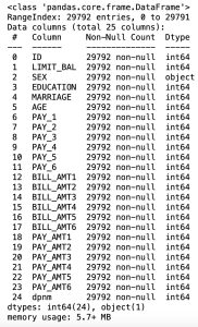
df.info()

In the Pandas library, the info() method prints summary information about the DataFrame.

Data Processing

Removing the unneccesary variables
Removing null values
Removing the duplicated values
Converting string variable(for example, sex variable) into numerical variable

df = df.drop('ID', axis=1)

# Checking missing values
df.isnull().sum()

There are no missing values in our dataset.

# Checking for the presence of duplicate values. If there exists, we have to remove the rows.
df = df.drop_duplicates()
print("The number of rows removed: %d." % (row_cnt0 - df.shape[0]))

The number of rows removed: 34

# Independent variable and dependent variable
X = df.drop('dpnm', axis=1)
y = df['dpnm']

Converting string variables into numerical variables

All the calculations are performed only with numbers. Thus, we need to convert the useful features into numbers. Feature Engineering is the process of transforming raw data into useful features that help us to understand our model better and increase its predictive power.

# encode variables with ordinal encoding
encoder = ce.OrdinalEncoder(cols=['SEX'])
X = encoder.fit_transform(X)
X0 = X.copy()
X.head()

Feature Selection

# Evaluating correlation of variables to prevent overfitting
plt.figure(figsize=(16, 16))
sns.heatmap(X.corr(),annot=True, cmap='BrBG_r')
plt.show()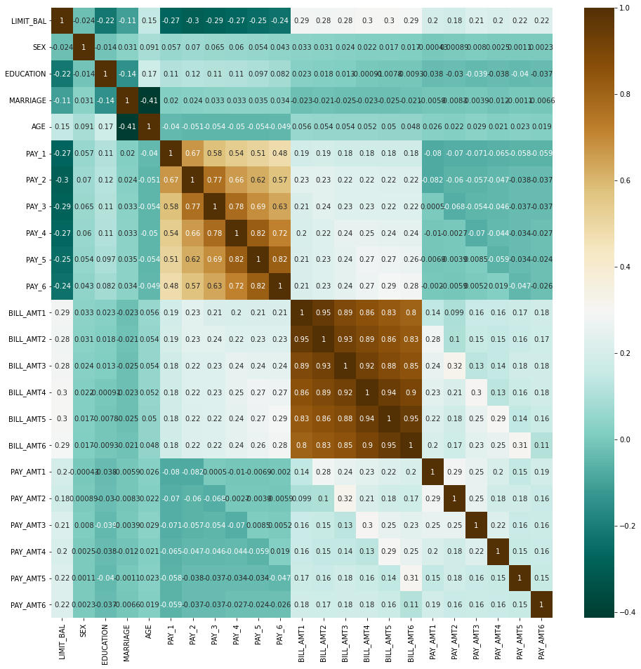

From the above correlation, variable “BILL_AMT1” has high positive correlations with variables “BILL_AMT2”, “BILL_AMT3”, “BILL_AMT4”, “BILL_AMT5”, “BILL_AMT6”. Therefore, we can remove 5 variables: “BILL_AMT2”, “BILL_AMT3”, “BILL_AMT4”, “BILL_AMT5”, “BILL_AMT6”.

X = X.drop(['BILL_AMT2', 'BILL_AMT3', 'BILL_AMT4', 'BILL_AMT5', 'BILL_AMT6'], axis=1)
X.head()

Train-Test Split

It is usually a good practice to keep 70% of the data in train dataset and the rest 30% in test dataset.

# data split
X_train, X_test, y_train, y_test = train_test_split(X, y, train_size = 0.7, test_size = 0.3, random_state = 50)

X_train

y_train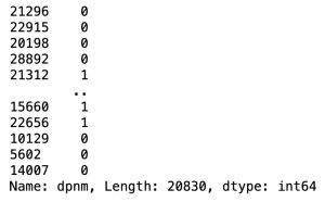

Building Decision Tree Classification Model

# Creating DecisionTreeClassifier model with criterion gini index
model = tree.DecisionTreeClassifier(criterion='gini', max_depth=3, random_state=100)

# Fitting train data
model.fit(X_train, y_train)

The output is: DecisionTreeClassifier(max_depth=3, random_state=100)

# Visualize decision-trees
plt.figure(figsize=(16,6))
tree.plot_tree(model)

# Predicting based on train data
y_pred_train = model.predict(X_train)

# Predicting based on test data
y_pred_test = model.predict(X_test)

Model Evaluation

Comparison of accuracies for train and test datasets

print('accuracy score for train dataset: %f.3' % accuracy_score(y_train, y_pred_train))
print('accuracy score for test dataset: %f.3' % accuracy_score(y_test, y_pred_test))

accuracy score for train dataset: 0.820979.3
accuracy score for test dataset: 0.822245.3

The accuracies are similar and thus, there is no overfitting.

Confusion Matrix

A confusion matrix is a performance evaluation tool in machine learning, representing the accuracy of a classification model. It displays the number of true positives, true negatives, false positives, and false negatives.

True positives (TP) occur when the model accurately predicts a positive data point.
True negatives (TN) occur when the model accurately predicts a negative data point.
False positives (FP) occur when the model predicts a positive data point incorrectly.
False negatives (FN) occur when the model mispredicts a negative data point.

# confusion matrix
from sklearn.metrics import confusion_matrix

confusion_m = confusion_matrix(y_test, y_pred_test)

sns.heatmap(confusion_m, annot=True, fmt='d', cmap='YlGnBu_r')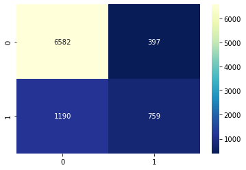

Classification Report

from sklearn.metrics import classification_report

print(classification_report(y_test, y_pred_test))

Prediction with Original Data(before removing some features)

# original data
X0

There are 23 independent variables.

# data split
X_train, X_test, y_train, y_test = train_test_split(X0, y, train_size = 0.7, test_size = 0.3, random_state = 50)

# Creating DecisionTreeClassifier model with criterion gini index
model = tree.DecisionTreeClassifier(criterion='gini', max_depth=3, random_state=100)

# Fitting train data
model.fit(X_train, y_train)

# Visualize decision-trees
plt.figure(figsize=(16,6))
tree.plot_tree(model) 

# Predicting based on train data
y_pred_train = model.predict(X_train)

# Predicting based on test data
y_pred_test = model.predict(X_test)

print('accuracy score for train dataset: %f.3' % accuracy_score(y_train, y_pred_train))
print('accuracy score for test dataset: %f.3' % accuracy_score(y_test, y_pred_test))

accuracy score for train dataset: 0.820979.3
accuracy score for test dataset: 0.822245.3

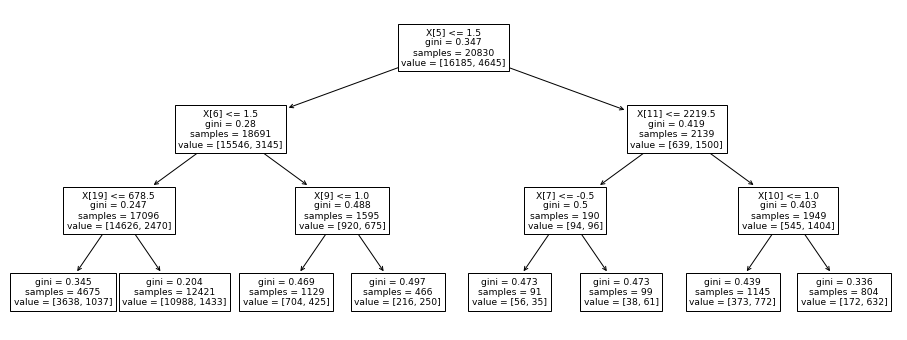
We can know that the accuracies after removing of some features by correlation analysis are almost the same as those before removing.

Therefore, it is better to use the model by removing some features to reduce calculation time.

Problem Statement

Data

Comments

Leave a Reply Cancel reply