Table of Contents
- Definition
- Types of SVM(Support Vector Machine)
- Formulation
- Analysis Steps
- Classification problem by SVM
Definition
In machine learning, support vector machines (SVMs, also support vector networks) are supervised max-margin models with associated learning algorithms that analyze data for classification and regression analysis.
A support vector is a data point or node lying closest to the decision boundary or hyperplane. These points play a vital role in defining the decision boundary and the margin of separation.
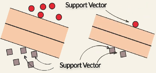
In addition to performing linear classification, SVMs can efficiently perform a non-linear classification using what is called the kernel trick, implicitly mapping their inputs into high-dimensional feature spaces. Being max-margin models, SVMs are resilient to noisy data (for example, mis-classified examples). SVMs can also be used for regression tasks, where the objective becomes 𝜖-sensitive.
Types of SVM(Support Vector Machine)
There are two different types of SVMs, each used for different things:
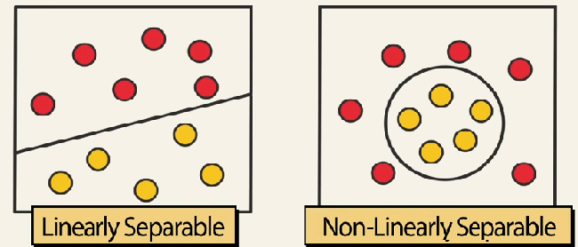
- Linear SVM(Simple SVM): Typically used for linear regression and classification problems.
- Kernel SVM: Has more flexibility for non-linear data because we can add more features to fit a hyperplane instead of a two-dimensional space.
Formulation
Support Vector Machines (SVM) is a supervised machine learning algorithm used for classification and regression tasks. The formulation of SVM involves finding the optimal hyperplane that separates data points of different classes with the maximum margin. Here’s the basic formulation:
Input Data: $\{(x_i, y_i)\}_{i=1}^{n}$, where $x_i$ represents the feature vector of the $i$-th sample, and $y_i$ represents the corresponding class label ($y_i \in \{-1, +1\}$ for binary classification).
Objective: The objective of SVM is to find the hyperplane $w \cdot x + b = 0$ that best separates the data points into two classes while maximizing the margin.
Formulation: Mathematically, the optimization problem can be formulated as:
\begin{align*}
\min_{w, b} & \quad \frac{1}{2} \|w\|^2 \\
\text{subject to} & \quad y_i(w \cdot x_i + b) \geq 1 \quad \text{for all } i = 1, \ldots, n
\end{align*}
This formulation ensures that the hyperplane separates the data with a margin of at least $\frac{1}{\|w\|}$. The points closest to the hyperplane, known as support vectors, lie on the boundary and define the margin.
Optimization: The optimization problem is typically solved using techniques like gradient descent or specialized quadratic programming solvers.
Kernel Trick (for Non-linear Separable Data): SVM can be extended to handle non-linearly separable data by mapping the input space into a higher-dimensional feature space using a kernel function $K(x, x’)$. Common choices for kernel functions include linear, polynomial, radial basis function (RBF), and sigmoid kernels.
The decision function then becomes:
\[
f(x) = \text{sign}\left(\sum_{i=1}^{n} \alpha_i y_i K(x, x_i) + b\right)
\]
where $\alpha_i$ are the Lagrange multipliers obtained from the optimization process.
Regularization: In practice, SVM often incorporates a regularization parameter $C$, which controls the trade-off between maximizing the margin and minimizing the classification error on the training data.
This formulation of SVM provides a powerful framework for finding a decision boundary that generalizes well to unseen data.
Analysis Steps
Here are the key steps to understand a our model:
- Data Collection: Gather the dataset containing the relevant information we want to model.
- Data Visualization and Data preprocessing:
- Data cleaning: Check for missing values and outliers.Handle them appropriately by imputing missing data or removing outliers
- Feature Selection/Engineering: Determine which independent variable are relevant for our model. we might need to transform or engineer features to make them suitable for regresion
- Assumption Check: If the given assumptions is not satisfied, we may need to apply transformations or consider different modeling techniques.
- Split Data: Divide our dataset into a training set and testing set. The training set is used to train the model and the testing set is sued to evaluate its preformance.
There are several methods for spliting datasets for machine learning and data analysis, Each method serves different purpose and has its advantages and disadvantages. Here are some comon dataset splitting methods along with step by step explanations for each:- Train-test Split(Holdout Method) – purpose to create two seperate sets, one for training and one for testing the mocel
Steps:- Randomly shuffle the dataset to ensure teh data is well distributed.
- Split the data into two parts, typically with a ratio like 70-30 or 80-20, where one part is for training and the other for testing
- Train our machine learning model on the training set
- Evaluate the model performance on the test set
K-Fold Cross Validation: Purpose to assess the model’s performance by training and testing it on different subsets of the data. steps: A. Divide the dataset into K equal sized folds B. For each fold(1 to K) treat it as a test set and the remaining K-1 folds as the training set. C. Train and evaluate the model on each of the K iterations. D. Calculate performance metrics(accuracy) by averaging the results from all iterations.
startified Sampling: purpose to ensure that the proportion of different classes in the dataset is maintained in teh train and test sets steps: A. Identify the target variable B. Stratify the data by the target variable to create representative subsets. C. perform a train_test split on these stratified subsets to maintain class balance in both sets
Time series split: purpose for time series data where the order of data oints matter steps A. sort the dataset based on the time or date variable B. Divide the data into training and testing sets such that the training set consists of past data and the testing set contains future data. - Leave one out cross validation – Purpose to leave out a single data point as the test set in each iteration. Steps: For each data point in the dataset, create a training set with all other data points. Train and test the model for each data point separately. Calculate the performance metrics based on the predictions from each iteration.
Group k-fold cross validation:purpose to accouont for groups or slusters in the data
Steps:- Randomly sample data points with replacement to create multiple bootstrap samples.
- Train and evaluate the model on each bootstrap sample.
- Calculate performance metrics based on the results of each sample.
- Train-test Split(Holdout Method) – purpose to create two seperate sets, one for training and one for testing the mocel
- Model Building:
- Choose the model: select either 3 types of models according to the values of dependent variable: binomial or multinomial, ordinal
- Fit the model: use the training data to estimate the coefficients that maximizes the likelihood of observing the data given
- Model Evaluation:
If our problem is Regression problem, use appropiate metrics like Mean Squared Error(MSE), Root Mean Squared Error(RMSE) or R-squared to evaluate how well our model fits.
If our problem is Classification problem, use appropiate metrics like acuracy, precision, recall, f1 Score, AUC-ROC or AUC-PR to evaluate how well our model fits.
Classification Problem by SVM
Problem Statement
The Human Activity Recognition database was built from the recordings by smartphone with embedded inertial sensors.
Here, we are going to classify activities into one of the six activities(WALKING, WALKING_UPSTAIRS, WALKING_DOWNSTAIRS, SITTING, STANDING, LAYING) performed.
Data
- Triaxial acceleration from the accelerometer (total acceleration) and the estimated body acceleration.
- Triaxial Angular velocity from the gyroscope.
- A 561-feature vector with time and frequency domain variables.
- Its activity label.
- An identifier of the subject who carried out the experiment.
Import Necessary Libraries
NumPy is a Python library used for working with arrays. It also has functions for working in domain of linear algebra, fourier transform, and matrices. NumPy can be used to perform a wide variety of mathematical operations on arrays. It adds powerful data structures to Python that guarantee efficient calculations with arrays and matrices and it supplies an enormous library of high-level mathematical functions that operate on these arrays and matrices.
Pandas is a Python library used for working with data sets. It has functions for analyzing, cleaning, exploring, and manipulating data. Pandas is a fast, powerful, flexible and easy to use open source data analysis and manipulation tool, built on top of the Python programming language.
Matplotlib is a comprehensive library for creating static, animated, and interactive visualizations in Python. Matplotlib makes easy things easy and hard things possible. Create publication quality plots. Make interactive figures that can zoom, pan, update. Customize visual style and layout.
Seaborn is a Python data visualization library based on matplotlib. It provides a high-level interface for drawing attractive and informative statistical graphics. It builds on top of matplotlib and integrates closely with pandas data structures. Seaborn helps we explore and understand our data.
Scikit-learn is probably the most useful library for machine learning in Python. The sklearn library contains a lot of efficient tools for machine learning and statistical modeling including classification, regression, clustering and dimensionality reduction.
# Supress Warnings
import warnings
warnings.filterwarnings('ignore')

# import the numpy and pandas packages
import numpy as np
import pandas as pd

# to visualize data
import matplotlib.pyplot as plt
import seaborn as sns

# to split arrays or matrices into random train and test subsets
from sklearn.model_selection import train_test_split
from sklearn.metrics import accuracy_score
from sklearn.model_selection import cross_val_score, KFold

# to import Support Vector Classifier model
from sklearn.svm import SVC

# import category encoders
# !pip install category_encoders
import category_encoders as ce
from sklearn.preprocessing import StandardScaler
Data Collection
# data source
url = "./SVM_dataset.csv"
# reading data
df = pd.read_csv(url)
df.head()
row_cnt0 = df.shape[0]
print("The number of rows : %d.\nThe number of columns is : %d." % (row_cnt0, df.shape[1]))
The number of rows: 10299
The number of columns is: 563
# data information
df.info()
In the Pandas library, the info() method prints summary information about the DataFrame.

Data Processing
- Removing the unneccesary variables
- Removing null values
- Removing the duplicated values
# Checking missing values
df.isnull().sum()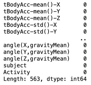
# Removing Null values
df = df.dropna(how='any',axis=0)
row_cnt1 = df.shape[0]
print("The number of rows deleted : %d" % (row_cnt0 - row_cnt1))
The number of rows deleted: 0
There are no missing values in our dataset.
# Checking for the presence of duplicate values. If there exists, we have to remove the rows.
df = df.drop_duplicates()
print("The number of rows removed: %d." % (row_cnt0 - df.shape[0]))
The number of rows removed: 0
There are no the duplicated values.
Visualizing of Target Variable(Dependent Variable)
# Visualizing frequency of target variable
plt.figure(figsize=(16, 6))
sns.countplot(x ='Activity', data = df)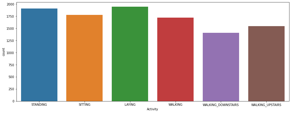
# Independent variable and dependent variable
X = df.drop('Activity', axis=1)
y = df['Activity']
y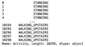
Converting string variables into numerical variables
All the calculations are performed only with numbers. Thus, we need to convert the useful features into numbers. Feature engineering is the process of transforming raw data into useful features that help us to understand our model better and increase its predictive power.
# encode variables with ordinal encoding
# In our case, only target variable has categorical values.
encoder = ce.OrdinalEncoder(cols=['Activity'])
y = encoder.fit_transform(y)
y.head()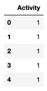
Normalizing the data can lead to faster training and better performance of the model. To address skewness in the data: Normalization in machine learning can help to address skewness in the data, which can be caused by outliers or by the data being distributed in a non-normal way.
# Standardizing input(independent) variables
scalar = StandardScaler()
scaled_X = scalar.fit_transform(X)
Train-Test Split
It is usually a good practice to keep 70% of the data in train dataset and the rest 30% in test dataset.
# data split
X_train, X_test, y_train, y_test = train_test_split(X, y, train_size = 0.7, test_size = 0.3, random_state = 50)
X_train
y_train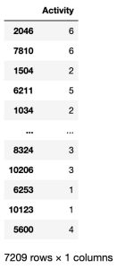
Building SVC(Support Vector Classifier) Model with Kernel “RBF”
# Creating SVC model
model = SVC(kernel='rbf')
# Fitting train data
model.fit(X_train, y_train)# Predicting based on train data
y_pred_train = model.predict(X_train)# Predicting based on test data
y_pred_test = model.predict(X_test)Model Evaluation
Comparison of accuracies for train and test datasets
print('accuracy score for train dataset: %f.3' % accuracy_score(y_train, y_pred_train))
print('accuracy score for test dataset: %f.3' % accuracy_score(y_test, y_pred_test))accuracy score for train dataset: 0.955334.3
accuracy score for test dataset: 0.957605.3
The accuracies are similar and thus, there is no overfitting.
During the use of kernel RBF(Gaussian kernel, or called Radius Basis Functions), our model gives very high accuracy of result.
Confusion Matrix
A confusion matrix is a performance evaluation tool in machine learning, representing the accuracy of a classification model. It displays the number of true positives, true negatives, false positives, and false negatives.
- True positives (TP) occur when the model accurately predicts a positive data point.
- True negatives (TN) occur when the model accurately predicts a negative data point.
- False positives (FP) occur when the model predicts a positive data point incorrectly.
- False negatives (FN) occur when the model mispredicts a negative data point.
# confusion matrix
from sklearn.metrics import confusion_matrix
confusion_m = confusion_matrix(y_test, y_pred_test)sns.heatmap(confusion_m, annot=True, fmt='d', cmap='YlGnBu_r')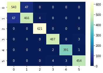
Classification Report
from sklearn.metrics import classification_report
print(classification_report(y_test, y_pred_test))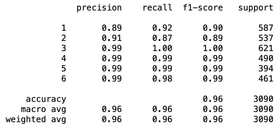
Building SVC(Support Vector Classifier) Model with Kernel “Linear”
# Creating SVC model
model = SVC(kernel='linear')
# Fitting train data
model.fit(X_train, y_train)
# Predicting based on train data
y_pred_train = model.predict(X_train)
# Predicting based on test data
y_pred_test = model.predict(X_test)
print('accuracy score for train dataset: %f.3' % accuracy_score(y_train, y_pred_train))
print('accuracy score for test dataset: %f.3' % accuracy_score(y_test, y_pred_test))
accuracy score for train dataset: 0.993064.3
accuracy score for test dataset: 0.985113.3
K-fold Cross Validation
In K-Fold Cross Validation, we split the dataset into k number of subsets (known as folds) then we perform training on the all the subsets but leave one(k-1) subset for the evaluation of the trained model. In this method, we iterate k times with a different subset reserved for testing purpose each time.
If the k-fold number is 5, the ratio of train and test data is (5-1)/5=80% and 1/5=20%.
# Creating SVC model with kernel "linear"
model = SVC(kernel='linear')

num_folds = 5
kf = KFold(n_splits=num_folds, shuffle=True, random_state=42)

cross_val_results = cross_val_score(model, X, y, cv=kf)

print(f'Cross-Validation Results (Accuracy): {cross_val_results}')
print(f'Mean Accuracy: {cross_val_results.mean()}')
Cross-Validation Results (Accuracy): [0.9868932 0.98446602 0.98495146 0.99174757 0.98154444]
Mean Accuracy: 0.9859205382950531
# Creating SVC model with kernel "RBF"
model = SVC(kernel='rbf')

num_folds = 5
kf = KFold(n_splits=num_folds, shuffle=True, random_state=42)

cross_val_results = cross_val_score(model, X, y, cv=kf)

print(f'Cross-Validation Results (Accuracy): {cross_val_results}')
print(f'Mean Accuracy: {cross_val_results.mean()}')
Conclusion
In our problem, Support Vector Classifier with linear kernel gives higher accuracy than that of RBF kernel and the calculation time is faster, also. Therefore, it is better to use SVC with linear kernel if possible.

Leave a Reply