Table of Contents
- Definition
- Assumptions
- Types of Linear Regression
- Formulation
- Analysis Steps
- Simple linear regression(Sales Prediction Problem)
Definition
In statistics, linear regression is a statistical model which estimates the linear relationship between a scalar response(known as dependent variable or target variable) and one or more explanatory variables (known as independent variables or predictor variables). Linear regression is an analytics procedure that can generate predictions by using an easily interpreted mathematical formula.
Difference between classification and regression: Classification and regression are machine learning tasks, but they differ in output. Classification predicts discrete labels or categories, while regression predicts continuous numerical values.
Linear Regression is the supervised Machine Learning model in which the model finds the best fit linear line between the independent and dependent variable i.e it finds the linear relationship between the dependent and independent variable. Supervised learning is a paradigm in machine learning where input objects and a desired output value train a model. The training data is processed, building a function that maps new data on expected output values.
Assumptions
Given below are the basic assumptions that a linear regression model makes regarding a dataset on which it is applied:
- Linear relationship: The relationship between response and feature variables should be linear. The linearity assumption can be tested using scatter plots. As shown below, 1st figure represents linearly related variables whereas variables in the 2nd and 3rd figures are most likely non-linear. So, 1st figure will give better predictions using linear regression.
- Little or no multi-collinearity: It is assumed that there is little or no multicollinearity in the data. Multicollinearity occurs when the features (or independent variables) are not independent of each other.
- Little or no autocorrelation: Another assumption is that there is little or no autocorrelation in the data. Autocorrelation occurs when the residual errors are not independent of each other. We can refer here for more insight into this topic.
- No outliers: We assume that there are no outliers in the data. Outliers are data points that are far away from the rest of the data. Outliers can affect the results of the analysis.
- Homoscedasticity: Homoscedasticity describes a situation in which the error term (that is, the “noise” or random disturbance in the relationship between the independent variables and the dependent variable) is the same across all values of the independent variables. As shown below, figure 1 has homoscedasticity while Figure 2 has heteroscedasticity.
Types of Linear Regression
There are two main types of linear regression:
- Simple linear regression: This involves predicting a dependent variable based on a single independent variable.
- Multiple linear regression: This involves predicting a dependent variable based on multiple independent variables.
Formulation
Linear regression is a fundamental statistical technique used to model the relationship between a dependent variable and one or more independent variables.
The simplest form, simple linear regression, involves two variables: one dependent (Y) and one independent (X). The relationship is modeled through an equation, Y = a + bX, where ‘b’ is the slope of the regression line, showing how much Y changes for each unit increase in X, and ‘a’ is the y-intercept, indicating the value of Y when X is zero. This method is widely used in data analysis to predict outcomes, understand relationships, and drive decision-making processes across various fields such as economics, engineering, and the social sciences.
By analyzing the coefficients ‘a’ and ‘b’, researchers can infer trends and make predictions based on the values of the independent variables.
Analysis Steps
Here are the key steps to understand a linear regression model:
- Data Collection: Gather the dataset containing the relevant information we want to model. For simple linear regresion we typically have one dependent variable and one independent variable. In multiple linear regression we have multiple independent variables.
- Data preprocessing:
- Data cleaning: Check for missing values and outliers.Handle them appropriately by imputing missing data or removing outliers
- Feature Selection/Engineering: Determine which independent variable are relevant for our model. we might need to transform or engineer features to make them suitable for regresion
- Data Visualization: Visualize the data by creating a scatterplot of the dependent variable against the independent variables to get an initial sens of the relationship.
- Assumption Check: Linear regression makes several assumptions, including linearity, independence of errors, homoscedasticity, and normality of errors. We should check if our data satisfies these assumptions. If not, we may need to apply transformations or consider different modeling techniques.
- Split Data: Divide our dataset into a training set and testing set. The training set is used to train the model and the testing set is sued to evaluate its preformance.
There are several methods for spliting datasets for machine learning and data analysis, Each method serves different purpose and has its advantages and disadvantages. Here are some comon dataset splitting methods along with step by step explanations for each:- Train-test Split(Holdout Method) – purpose to create two seperate sets, one for training and one for testing the mocel
Steps:- Randomly shuffle the dataset to ensure teh data is well distributed.
- Split the data into two parts, typically with a ratio like 70-30 or 80-20, where one part is for training and the other for testing
- Train our machine learning model on the training set
- Evaluate the model performance on the test set
K-Fold Cross Validation: Purpose to assess the model’s performance by training and testing it on different subsets of the data. steps: A. Divide the dataset into K equal sized folds B. For each fold(1 to K) treat it as a test set and the remaining K-1 folds as the training set. C. Train and evaluate the model on each of the K iterations. D. Calculate performance metrics(accuracy) by averaging the results from all iterations.
Startified Sampling: purpose to ensure that the proportion of different classes in the dataset is maintained in teh train and test sets steps: A. Identify the target variable B. Stratify the data by the target variable to create representative subsets. C. perform a train_test split on these stratified subsets to maintain class balance in both sets
Time series split: purpose for time series data where the order of data oints matter steps A. sort the dataset based on the time or date variable B. Divide the data into training and testing sets such that the training set consists of past data and the testing set contains future data. - Leave one out cross validation – Purpose to leave out a single data point as the test set in each iteration. Steps: For each data point in the dataset, create a training set with all other data points. Train and test the model for each data point separately. Calculate the performance metrics based on the predictions from each iteration.
Group k-fold cross validation:purpose to accouont for groups or slusters in the data
Steps:- Randomly sample data points with replacement to create multiple bootstrap samples.
- Train and evaluate the model on each bootstrap sample.
- Calculate performance metrics based on the results of each sample.
- Train-test Split(Holdout Method) – purpose to create two seperate sets, one for training and one for testing the mocel
- Model Building:
- Choose the model: select either simple liner regression or multiple linear regression
- Fit the model: use the training data to estimate the coefficients that minimize the sum of squared differences between the observed and predicted values
- Interpret the Coefficients: Understand the meaning of the coefficients for each independent variable. They represent the change in the dependent variable for a one unit change in the corresponding independent variable, assuming all other variables are held constant.
- Model Evaluation:
- Assess Model fit: Use appropiate metrics like Mean Squared Error(MSE), Root Mean Squared Error(RMSE) or R-squared to evaluate how well our model fits the training data.
- Test the model: Apply the model to the testing set to assess its predictive accuracy on unseen data
- Model Interpretation:
- Coefficient Significance: Determine if the coefficients are statistically significant using hypothesis tests
- Coefficient Interpretation: interpret the coefficients in the context of our problem to make meaningful conclusions.
- Prediction and Inference: Use the model to make predictions or draw inferences about the relationship between the dependent and independent variables.
- Model Deployment: if the model performs well and is valuable it can be deployed in production for real world predictions.
- Regularization: In some cases we might apply regularization techniques like Ridge or lasso regression to prevent overfitting or handle multicollinearity.
- Continuous Imporvement: As new data becomes available we may need to retrain the model to keep it accurate and relevant.
Simple linear regression(Sales Prediction Problem)
Problem Statement
Build a model which predicts sales based on the money spent on different platforms for marketing.
Data
Use the advertising dataset given in ISLR and analyse the relationship between ‘TV advertising’ and ‘sales’ using a simple linear regression model.
We are going to build a linear regression model to predict Sales using an appropriate predictor variable.
Import Necessary libraries
NumPy is a Python library used for working with arrays. It also has functions for working in domain of linear algebra, fourier transform, and matrices. NumPy can be used to perform a wide variety of mathematical operations on arrays. It adds powerful data structures to Python that guarantee efficient calculations with arrays and matrices and it supplies an enormous library of high-level mathematical functions that operate on these arrays and matrices.
Pandas is a Python library used for working with data sets. It has functions for analyzing, cleaning, exploring, and manipulating data. Pandas is a fast, powerful, flexible and easy to use open source data analysis and manipulation tool, built on top of the Python programming language.
Matplotlib is a comprehensive library for creating static, animated, and interactive visualizations in Python. Matplotlib makes easy things easy and hard things possible. Create publication quality plots. Make interactive figures that can zoom, pan, update. Customize visual style and layout.
Seaborn is a Python data visualization library based on matplotlib. It provides a high-level interface for drawing attractive and informative statistical graphics. It builds on top of matplotlib and integrates closely with pandas data structures. Seaborn helps we explore and understand our data.
Scikit-learn is probably the most useful library for machine learning in Python. The sklearn library contains a lot of efficient tools for machine learning and statistical modeling including classification, regression, clustering and dimensionality reduction.
Statsmodels is a Python package that allows users to explore data, estimate statistical models, and perform statistical tests. Statsmodels is built on top of NumPy, SciPy, and matplotlib, but it contains more advanced functions for statistical testing and modeling that we won’t find in numerical libraries like NumPy or SciPy.
# Supress Warnings
import warnings
warnings.filterwarnings('ignore')

# import the numpy and pandas packages
import numpy as np
import pandas as pd

# to visualize data
import matplotlib.pyplot as plt
import seaborn as sns

# to split arrays or matrices into random train and test subsets
from sklearn.model_selection import train_test_split

# to use linear regression model from sklearn package
import statsmodels.api as sm
Data Collection
# data source
url = "./LinearRegression_advertising.csv"
# reading data
df = pd.read_csv(url)
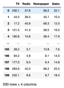
dfWe have a data set of 200 rows consisting of 4 columns.
# data information
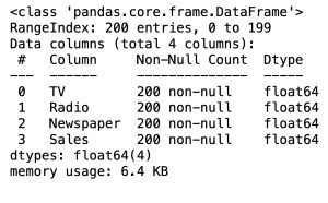
df.info()
In the Pandas library, the info() method prints summary information about the DataFrame.
Data Processing
# Checking Null values
df.isnull().sum()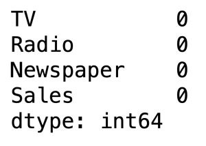
There are no NULL values in the dataset, hence it is clean.
# Outlier Analysis
fig, axs = plt.subplots(3, figsize = (5,5))
sns.boxplot(df['TV'], ax = axs[0])
sns.boxplot(df['Radio'], ax = axs[1])
sns.boxplot(df['Newspaper'], ax = axs[2])
plt.tight_layout()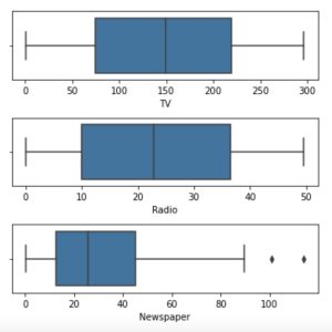
There are no considerable outliers present in the data.
Feature Selection
Univariate Analysis: Sales (Target Variable)
sns.boxplot(df['Sales'])
plt.show()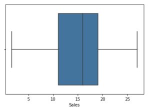
Here, we consider how Sales are related with other variables using scatter plot.
fig, axs = plt.subplots(ncols=3, figsize=(16, 4))
sns.scatterplot(x='TV', y='Sales', data=df, ax = axs[0])
sns.scatterplot(x='Radio', y='Sales', data=df, ax = axs[1])
sns.scatterplot(x='Newspaper', y='Sales', data=df, ax = axs[2])
plt.show()
Let’s consider the correlation between different variables to select feature to use.
# correlation analysis
sns.heatmap(df.corr(), cmap="YlGnBu", annot = True)
plt.show()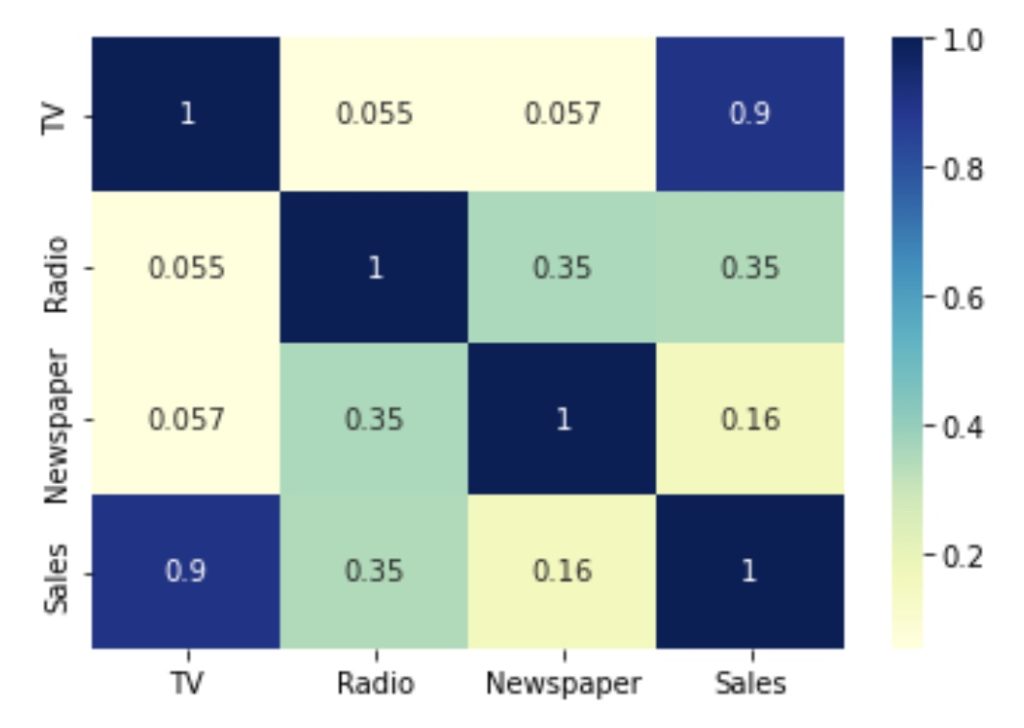
From the above graph, the variable TV seems to be most correlated with Sales. Therefore, we can select TV as our feature variable.
Train-Test Split
It is usually a good practice to keep 70% of the data in train dataset and the rest 30% in test dataset.
# We first assign the feature variable, TV to the variable X and the response variable, Sales, to the variable y.
X = df['TV']
y = df['Sales']

# data split
X_train, X_test, y_train, y_test = train_test_split(X, y, train_size = 0.7, test_size = 0.3, random_state = 50)X_train.head()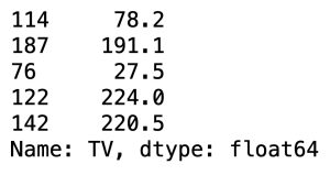
y_train.head()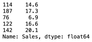
Building Linear Regression Model
By default, the statsmodels library fits a line on the dataset which passes through the origin. But in order to have an intercept, we need to manually use the add_constant attribute of statsmodels. And once we’ve added the constant to our X_train dataset, we can go ahead and fit a regression line using the OLS (Ordinary Least Squares) attribute of statsmodels as shown below.
OLS or Ordinary Least Squares is a useful method for evaluating a linear regression model.
# Add a constant to get an intercept
X_train_sm = sm.add_constant(X_train)

# Fit the resgression line using 'OLS'.
lr = sm.OLS(y_train, X_train_sm).fit()
# Print the parameters, i.e. the intercept and the slope of the regression line fitted
lr.params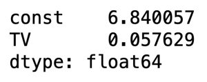
# Performing a summary operation lists out all the different parameters of the regression line fitted
print(lr.summary())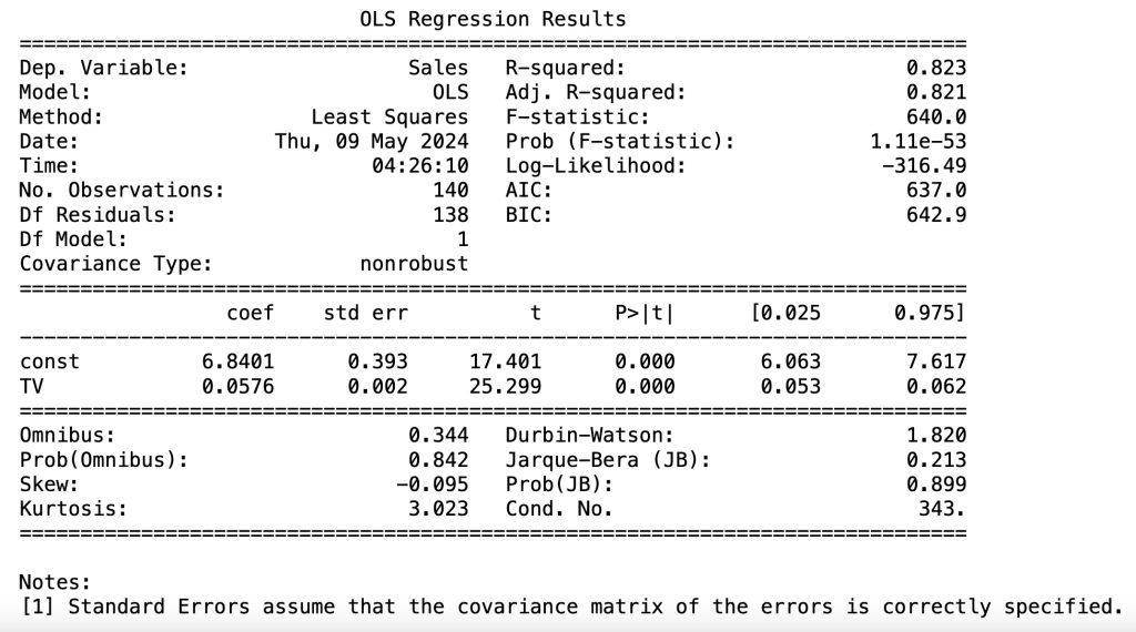
Model Evaluation and Interpretation with train data
- The coefficient for TV is 0.0576, with a very low p value( <
0.05).
The coefficient is statistically significant. So the association is not purely by chance. - R – squared is 0.823.
Meaning that 82.3% of the variance in Sales is explained by TV. This is a decent R-squared value. - F statistic has a very low p value (practically low).
Meaning that the model fit is statistically significant, and the explained variance isn’t purely by chance.
The fit is significant. Let’s visualize how well the model fit the data.
From the parameters that we get, our linear regression equation becomes:
Sales = 6.8401 + 0.0576 × TV
# scatterplot and regression line for train data
plt.scatter(X_train, y_train)
plt.plot(X_train, 6.948 + 0.054*X_train, 'r')
plt.show()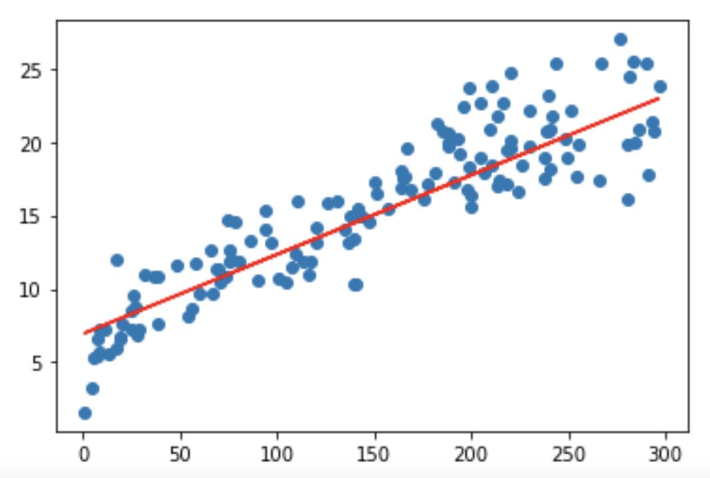
Residual analysis
To validate assumptions of the model, and hence the reliability for inference.
Distribution of the error terms: We need to check if the error terms are also normally distributed (which is infact, one of the major assumptions of linear regression), let us plot the histogram of the error terms and see what it looks like.
y_train_pred = lr.predict(X_train_sm)
res = (y_train - y_train_pred)
fig = plt.figure()
sns.distplot(res, bins = 15)
fig.suptitle('Error Terms', fontsize = 15) # Plot heading
plt.xlabel('y_train - y_train_pred', fontsize = 15) # X-label
plt.show()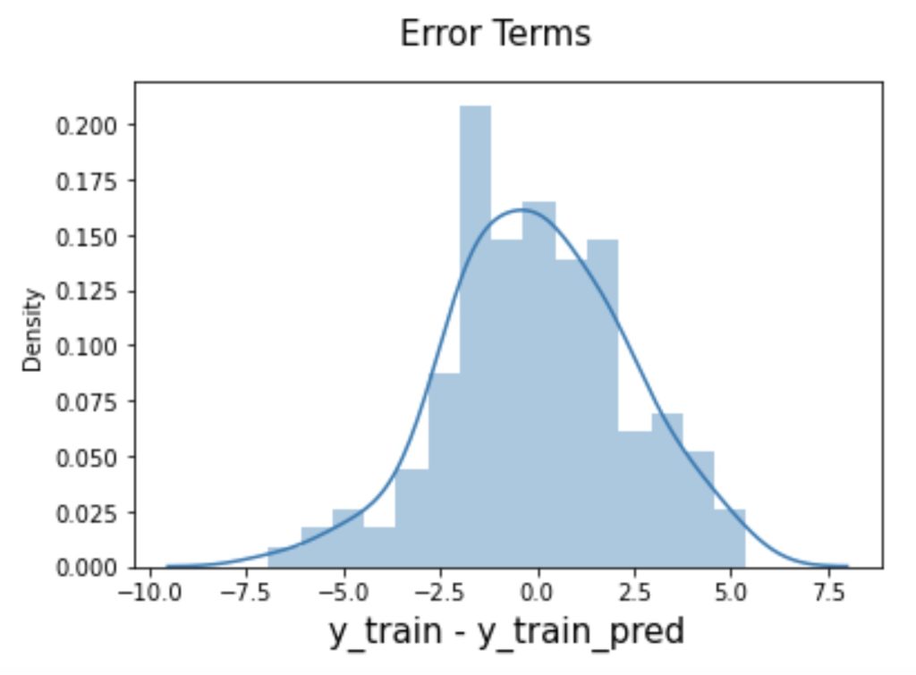
The residuals are following the normally distributed with a mean 0. All good!
Looking for patterns in the residuals
plt.scatter(X_train,res)
plt.show()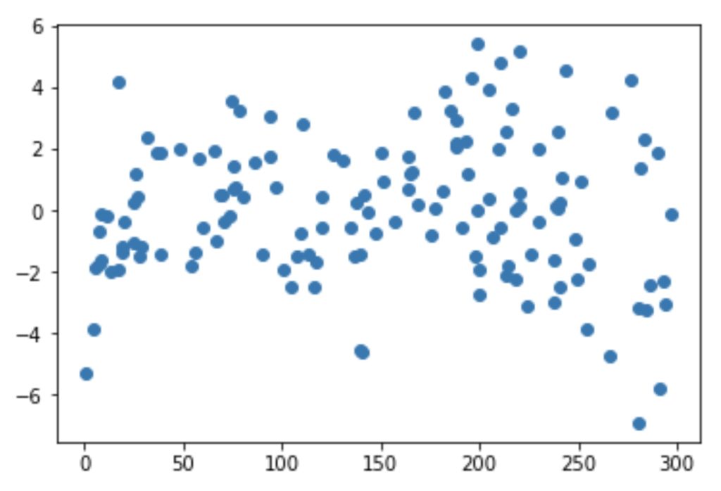
We are confident that the model fit isn’t by chance, and has decent predictive power. The normality of residual terms allows some inference on the coefficients.
As we can see, the regression line is a pretty good fit to the data
Model Evaluation for test data
Now that we have fitted a regression line on our train dataset, it’s time to make some predictions on the test data. For this, we first need to add a constant to the X_test data like we did for X_train and then we can simply go on and predict the y values corresponding to X_test using the predict attribute of the fitted regression line.
# Add a constant to X_test
X_test_sm = sm.add_constant(X_test)

# Predict the y values corresponding to X_test_sm
y_pred = lr.predict(X_test_sm)y_pred.head()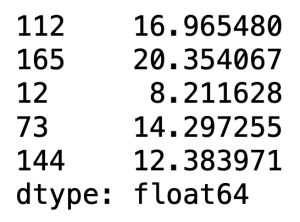
from sklearn.metrics import mean_squared_error
from sklearn.metrics import r2_score#Returns the mean squared error; we'll take a square root
np.sqrt(mean_squared_error(y_test, y_pred))The output is: 2.2488177561425107
Checking the R-squared on the test set
r_squared = r2_score(y_test, y_pred)
r_squared
The output is: 0.7596642945163175
Visualizing the fit on the test set
plt.scatter(X_test, y_test)
plt.plot(X_test, 6.948 + 0.054 * X_test, 'r')
plt.show()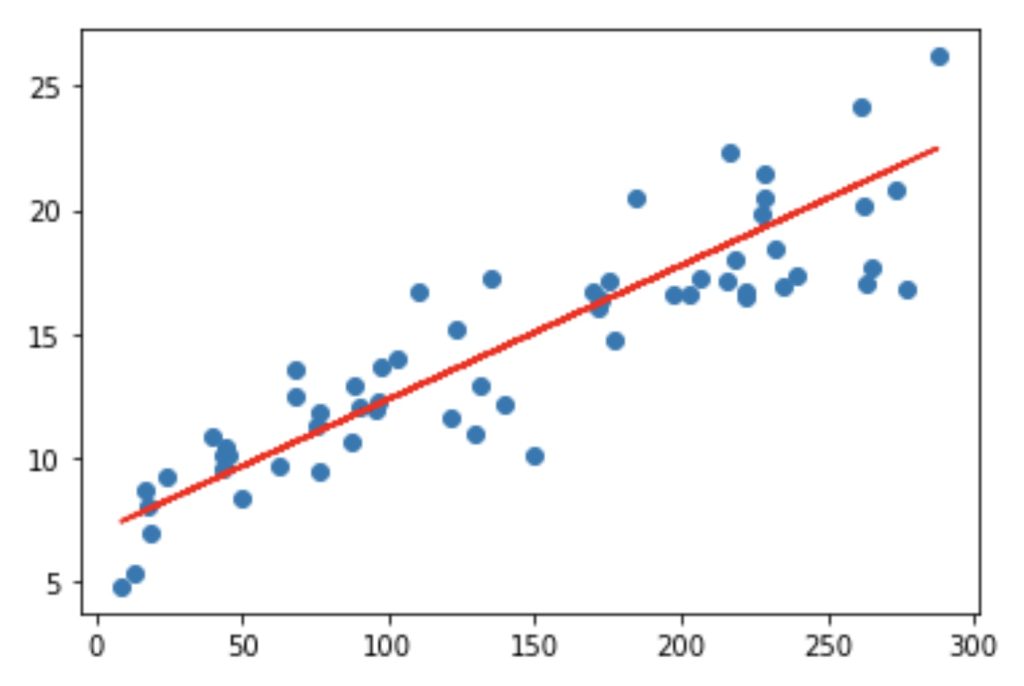
Conclusion
