Table of Contents
- Definition
- Formulation
- Analysis Steps
- Classification problem by Random Forests
Definition
Random forests or random decision forests is an ensemble learning method for classification, regression and other tasks that operates by constructing a multitude of decision trees at training time. For classification tasks, the output of the random forest is the class selected by most trees. For regression tasks, the mean or average prediction of the individual trees is returned.
Ensemble methods are techniques that aim at improving the accuracy of results in models by combining multiple models instead of using a single model. The combined models increase the accuracy of the results significantly.
Random Forest is a supervised machine learning algorithm made up of decision trees. Each decision tree is constructed using a random subset of the data set to measure a random subset of features in each partition. A decision tree is a decision support hierarchical model that uses a tree-like model of decisions and their possible consequences, including chance event outcomes, resource costs, and utility. It is one way to display an algorithm that only contains conditional control statements. And supervised learning is a paradigm in machine learning where input objects and a desired output value train a model. The training data is processed, building a function that maps new data on expected output values.
A decision tree is more simple and interpretable but prone to overfitting, but a random forest is complex and prevents the risk of overfitting. Random forest is a more robust and generalized performance on new data, widely used in various domains such as finance, healthcare, and deep learning.

Formulation
The vector \(x\) is composed of the features (independent variables), \(x_1, x_2, x_3, \ldots\), that are used for that task. The dependent variable, \(Y\), is the target variable that we are trying to understand.
\[
X = \begin{bmatrix}
x_1 \\
x_2 \\
\vdots \\
x_n
\end{bmatrix}
\]
Understanding of Ensemble Learning
Ensemble Learning
- Method that combines multiple learning algorithms to obtain performance improvements over its components
Random Forests are one of the most common examples of ensemble learning
Other commonly-used ensemble methods:
- Bagging: Multiple models on random subsets of data samples
- Random Subspace Method: Multiple models on random subsets of features
- Boosting: Train models iteratively, while making the current model focus on the mistakes of the previous ones by increasing the weight of misclassified samples
Step 1

Step 2

Step 3

Step 4
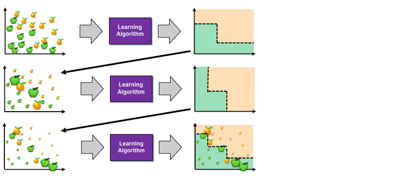
Step 6
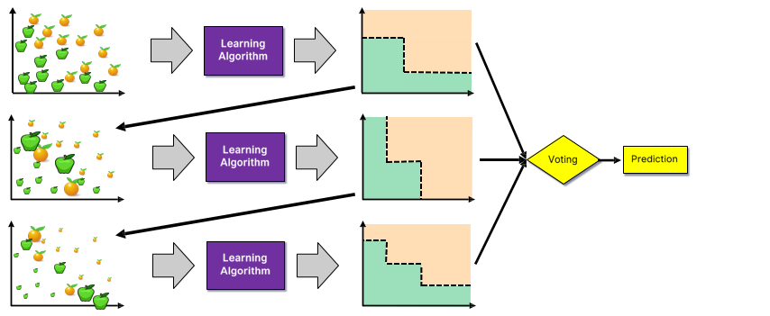
Random Forests
Random Forests are an ensemble learning method that employ decision tree learning to build multiple trees through bagging and random subspace method.

Bagging
Bagging repeatedly (B times) selects a random sample with replacement of the training set and fits trees to these samples. Here, B means the number of trees.
For b = 1, …, B:
- Sample, with replacement, n training examples from X, Y; call these Xb, Yb.
- Train a classification or regression tree fb on Xb, Yb.
Regression: After training, predictions for unseen samples x’ can be made by averaging the predictions from all the individual regression trees on x’
Classification: After training, predictions for unseen samples x’ take Majority vote.
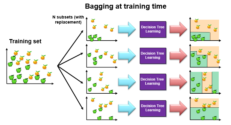
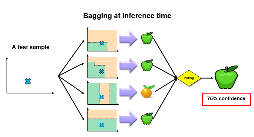
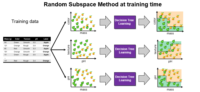
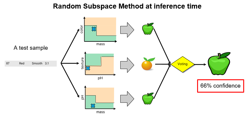
Random Subspace Method
The Random Subspace Method (RSM) is a technique used in ensemble learning, such as in random forests, to enhance model accuracy and robustness by training each model on a random subset of features.
This approach not only helps in managing high-dimensional data effectively by reducing dimensionality but also increases the diversity among the models in the ensemble, which is critical for reducing variance.
While RSM can make models more resistant to noise and irrelevant features, it may also lead to information loss since not all features are used in each model, necessitating careful tuning of parameters to balance diversity with the risk of omitting critical information.
Variable(Feature) Importance
Variable importance in random forests refers to the measure of how much a predictor variable contributes to the accuracy of a random forest model. This is calculated by considering the impact of each variable on the forest outcomes, including the number of times it’s selected in multiple trees, the number of times it splits an internal node, and the decrease in impurity resulting from splitting on that variable. Higher variable importance indicates that the variable is more influential in predicting the outcome.
Out-of-bag Error
Out-of-bag (OOB) error, also called out-of-bag estimate, is a method of measuring the prediction error of random forests, boosted decision trees, and other machine learning models utilizing bootstrap aggregating (bagging). Bagging uses subsampling with replacement to create training samples for the model to learn from. OOB error is the mean prediction error on each training sample xi, using only the trees that did not have xi in their bootstrap sample.
Since each out-of-bag set is not used to train the model, it is a good test for the performance of the model. The specific calculation of OOB error depends on the implementation of the model, but a general calculation is as follows.
- Find all models (or trees, in the case of a random forest) that are not trained by the OOB instance.
- Take the majority vote of these models’ result for the OOB instance, compared to the true value of the OOB instance.
- Compile the OOB error for all instances in the OOB dataset.
The bagging process can be customized to fit the needs of a model. To ensure an accurate model, the bootstrap training sample size should be close to that of the original set. Also, the number of iterations (trees) of the model (forest) should be considered to find the true OOB error. The OOB error will stabilize over many iterations so starting with a high number of iterations is a good idea.
Analysis Steps
Here are the key steps to understand a our model:
- Data Collection: Gather the dataset containing the relevant information we want to model.
- Data Visualization and Data preprocessing:
- Data cleaning: Check for missing values and outliers.Handle them appropriately by imputing missing data or removing outliers
- Feature Selection/Engineering: Determine which independent variable are relevant for our model. we might need to transform or engineer features to make them suitable for regresion
- Assumption Check: If the given assumptions is not satisfied, we may need to apply transformations or consider different modeling techniques.
- Split Data: Divide our dataset into a training set and testing set. The training set is used to train the model and the testing set is sued to evaluate its preformance.
There are several methods for spliting datasets for machine learning and data analysis, Each method serves different purpose and has its advantages and disadvantages. Here are some comon dataset splitting methods along with step by step explanations for each:- Train-test Split(Holdout Method) – purpose to create two seperate sets, one for training and one for testing the mocel
Steps:- Randomly shuffle the dataset to ensure teh data is well distributed.
- Split the data into two parts, typically with a ratio like 70-30 or 80-20, where one part is for training and the other for testing
- Train our machine learning model on the training set
- Evaluate the model performance on the test set
K-Fold Cross Validation: Purpose to assess the model’s performance by training and testing it on different subsets of the data. steps: A. Divide the dataset into K equal sized folds B. For each fold(1 to K) treat it as a test set and the remaining K-1 folds as the training set. C. Train and evaluate the model on each of the K iterations. D. Calculate performance metrics(accuracy) by averaging the results from all iterations.
startified Sampling: purpose to ensure that the proportion of different classes in the dataset is maintained in teh train and test sets steps: A. Identify the target variable B. Stratify the data by the target variable to create representative subsets. C. perform a train_test split on these stratified subsets to maintain class balance in both sets
Time series split: purpose for time series data where the order of data oints matter steps A. sort the dataset based on the time or date variable B. Divide the data into training and testing sets such that the training set consists of past data and the testing set contains future data. - Leave one out cross validation – Purpose to leave out a single data point as the test set in each iteration. Steps: For each data point in the dataset, create a training set with all other data points. Train and test the model for each data point separately. Calculate the performance metrics based on the predictions from each iteration.
Group k-fold cross validation:purpose to accouont for groups or slusters in the data
Steps:- Randomly sample data points with replacement to create multiple bootstrap samples.
- Train and evaluate the model on each bootstrap sample.
- Calculate performance metrics based on the results of each sample.
- Train-test Split(Holdout Method) – purpose to create two seperate sets, one for training and one for testing the mocel
- Model Building:
- Choose the model
- Fit the model
- Model Evaluation:
If our problem is Regression problem, use appropiate metrics like Mean Squared Error(MSE), Root Mean Squared Error(RMSE) or R-squared to evaluate how well our model fits.
If our problem is Classification problem, use appropiate metrics like acuracy, precision, recall, f1 Score, AUC-ROC or AUC-PR to evaluate how well our model fits.
Classification Problem by Random Forests
Problem Statement
We have the data of applicants who previously applied for the loan based on the property which is a Property Loan. The bank will decide whether to give a loan to the applicant based on some factors such as Applicant Income, Loan Amount, previous Credit History, Co-applicant Income, etc…
Here, we are going to predict the loan to be approved or to be rejected for an applicant. And we analyze variable(feature) importance.
Data
CSV file contains all the information. Here are the names of variables.
- Loan_ID: A unique loan ID
- Gender: Either øor feø
- Married: Weather Married(yes) or Not Marttied(No)
- Dependents: Number of persons depending on the client
- Education: Applicant Education(Graduate or Undergraduate)
- Self_Employed: Self-employed (Yes/No)
- ApplicantIncome: Applicant income
- CoapplicantIncome: Co-applicant income
- LoanAmount: Loan amount in thousands
- Loan_Amount_Term: Terms of the loan in months
- Credit_History: Credit history meets guidelines
- Property_Area: Applicants are living either Urban, Semi-Urban or Rural
- Loan_Status: Loan approved (Y/N)
Import Necessary Libraries
NumPy is a Python library used for working with arrays. It also has functions for working in domain of linear algebra, fourier transform, and matrices. NumPy can be used to perform a wide variety of mathematical operations on arrays. It adds powerful data structures to Python that guarantee efficient calculations with arrays and matrices and it supplies an enormous library of high-level mathematical functions that operate on these arrays and matrices.
Pandas is a Python library used for working with data sets. It has functions for analyzing, cleaning, exploring, and manipulating data. Pandas is a fast, powerful, flexible and easy to use open source data analysis and manipulation tool, built on top of the Python programming language.
Matplotlib is a comprehensive library for creating static, animated, and interactive visualizations in Python. Matplotlib makes easy things easy and hard things possible. Create publication quality plots. Make interactive figures that can zoom, pan, update. Customize visual style and layout.
Seaborn is a Python data visualization library based on matplotlib. It provides a high-level interface for drawing attractive and informative statistical graphics. It builds on top of matplotlib and integrates closely with pandas data structures. Seaborn helps we explore and understand our data.
Scikit-learn is probably the most useful library for machine learning in Python. The sklearn library contains a lot of efficient tools for machine learning and statistical modeling including classification, regression, clustering and dimensionality reduction.
# Supress Warnings
import warnings
warnings.filterwarnings('ignore')

# import the numpy and pandas packages
import numpy as np
import pandas as pd

# to visualize data
import matplotlib.pyplot as plt
import seaborn as sns

# to split arrays or matrices into random train and test subsets
from sklearn.model_selection import train_test_split
from sklearn.metrics import accuracy_score
from sklearn.preprocessing import StandardScaler

# to impute null values
from sklearn.impute import SimpleImputer, KNNImputer

# to import Random Forest Classifier
from sklearn.ensemble import RandomForestClassifier
Data Collection
# data source
url = "./RandomForest_data.csv"
# reading data
df = pd.read_csv(url)
df.head()
row_cnt0 = df.shape[0]
print("The number of rows : %d.\nThe number of columns is : %d." % (row_cnt0, df.shape[1]))
The number of rows: 614
The number of columns is: 13
# data information
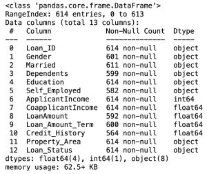
df.info()
In the Pandas library, the info() method prints summary information about the DataFrame.
Data Processing
- Removing the unneccesary variables
- Converting string variable(for example, Gender variable) into numerical variable
- Imputing null values
- Removing the duplicated values
Removing the unneccesary variables
df = df.drop('Loan_ID', axis=1)
df
Data Visualization
# Visualizing variables
plt.figure(figsize=(16, 16))
for i in range(1, len(df.columns)+1):
    plt.subplot(4, 3, i)
    if df.columns[i-1] in ['ApplicantIncome', 'CoapplicantIncome', 'LoanAmount', 'Loan_Amount_Term']:
        plt.plot(df[df.columns[i-1]])
        plt.ylabel(df.columns[i-1])
    else:
        ax = sns.countplot(x=df.columns[i-1], data=df)
        for container in ax.containers:
ax.bar_label(container) 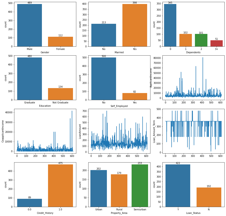
Converting string variable(for example, Gender variable) into numerical variable(except null values)
# Checking missing values
df.isnull().sum()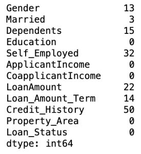
There are many missing values in our dataset.
# Saving names of categories in the specific column
encoded_label_names = {}
encoded_label_names['Gender'] = df['Gender'].unique()
encoded_label_names['Married'] = df['Married'].unique()
encoded_label_names['Dependents'] = df['Dependents'].unique()
encoded_label_names['Education'] = df['Education'].unique()
encoded_label_names['Self_Employed'] = df['Self_Employed'].unique()
encoded_label_names['Credit_History'] = df['Credit_History'].unique()
encoded_label_names['Property_Area'] = df['Property_Area'].unique()
encoded_label_names['Loan_Status'] = df['Loan_Status'].unique()
encoded_label_names
# Replacing categorical values into numbers
df1 = df.copy()
df1= df1.replace(encoded_label_names['Gender'][[0,1]],(1,0))
df1= df1.replace(encoded_label_names['Married'][[0,1]],(0,1))
df1= df1.replace(encoded_label_names['Dependents'][[0,1,2,3]],(0,1,2,3))
df1= df1.replace(encoded_label_names['Education'][[0,1]],(1,0))
df1= df1.replace(encoded_label_names['Self_Employed'][[0,1]],(0, 1))
df1= df1.replace(encoded_label_names['Property_Area'][[0,1,2]],(0,1,2))
df1= df1.replace(encoded_label_names['Loan_Status'][[0,1]],(1,0))
df1
Imputing Null Values
For various reasons, many real world datasets contain missing values, often encoded as blanks, NaNs or other placeholders. Such datasets however are incompatible with scikit-learn estimators which assume that all values in an array are numerical, and that all have and hold meaning. A basic strategy to use incomplete datasets is to discard entire rows and/or columns containing missing values. However, this comes at the price of losing data which may be valuable (even though incomplete). A better strategy is to impute the missing values, i.e., to infer them from the known part of the data.
Here, we are going to impute KNNImputer class.
The KNNImputer class provides imputation for filling in missing values using the k-Nearest Neighbors approach. By default, a euclidean distance metric that supports missing values, nan_euclidean_distances, is used to find the nearest neighbors. Each missing feature is imputed using values from n_neighbors nearest neighbors that have a value for the feature. The feature of the neighbors are averaged uniformly or weighted by distance to each neighbor. If a sample has more than one feature missing, then the neighbors for that sample can be different depending on the particular feature being imputed. When the number of available neighbors is less than n_neighbors and there are no defined distances to the training set, the training set average for that feature is used during imputation. If there is at least one neighbor with a defined distance, the weighted or unweighted average of the remaining neighbors will be used during imputation. If a feature is always missing in training, it is removed during transform.
# Imputing missing values
imputer = KNNImputer(n_neighbors=5)
df1 = pd.DataFrame(imputer.fit_transform(df1),columns = df1.columns)
df1
# Checking missing values
df1.isnull().sum()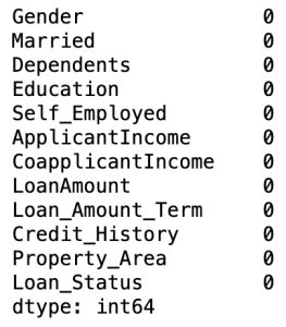
# Checking for the presence of duplicate values. If there exists, we have to remove the rows.
df1 = df1.drop_duplicates()
print("The number of rows removed: %d." % (row_cnt0 - df.shape[0]))
The number of rows removed: 0
# Spliting Predictor variables and target variable
X = df1.drop(columns=['Loan_Status'])
y = df1['Loan_Status']
X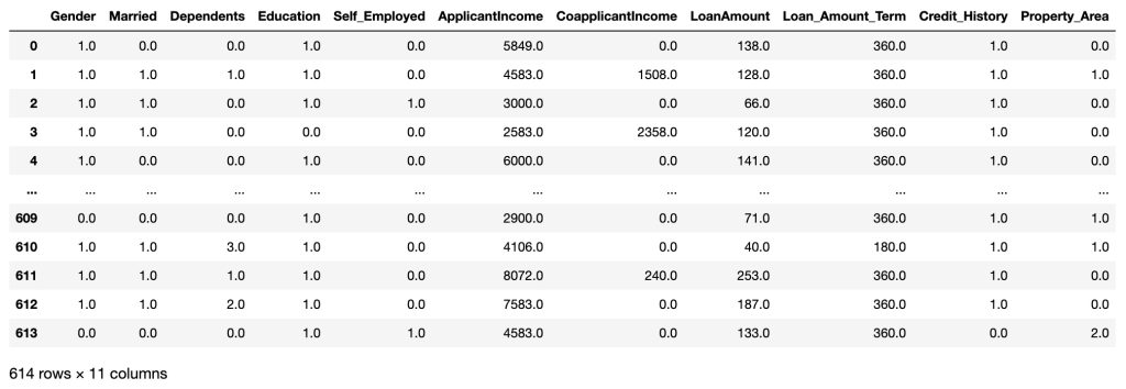
Feature Selection
# Evaluating correlation of variables to prevent overfitting
plt.figure(figsize=(16, 16))
sns.heatmap(X.corr(),annot=True, cmap='BrBG_r')
plt.show()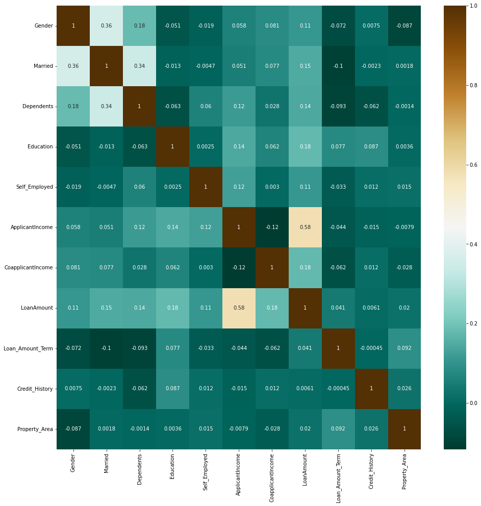
There are no considerable correlation coefficients.
Scaling Features
# Scaling features
scaler = StandardScaler()
X = scaler.fit_transform(X)
Train-Test Split
# data split
X_train, X_test, y_train, y_test = train_test_split(X, y, train_size = 0.8, random_state = 50)
X_train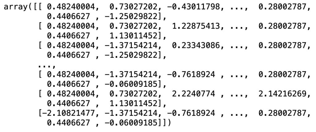
y_train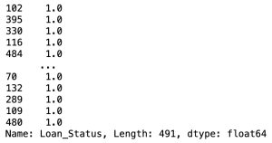
Building Random Forest Model
# Creating Random Forest Model
model = RandomForestClassifier(oob_score=True, random_state = 50)
# Fitting train data
model.fit(X_train, y_train)# Predicting based on test data
y_pred_test = model.predict(X_test)Model Evaluation
print('Accuracy score for test dataset: %f' % accuracy_score(y_test, y_pred_test))
print("OOB score :                      %f" % model.oob_score_)
oob_error = 1 - model.oob_score_
print("Out-of-bag error :               %f" % oob_error)
Accuracy score for test dataset: 0.780488
OOB score: 0.780041
Out-of-bag error: 0.219959
Confusion Matrix
A confusion matrix is a performance evaluation tool in machine learning, representing the accuracy of a classification model. It displays the number of true positives, true negatives, false positives, and false negatives.
- True positives (TP) occur when the model accurately predicts a positive data point.
- True negatives (TN) occur when the model accurately predicts a negative data point.
- False positives (FP) occur when the model predicts a positive data point incorrectly.
- False negatives (FN) occur when the model mispredicts a negative data point.
# confusion matrix
from sklearn.metrics import confusion_matrix

confusion_m = confusion_matrix(y_test, y_pred_test)sns.heatmap(confusion_m, annot=True, fmt='d', cmap='YlGnBu_r')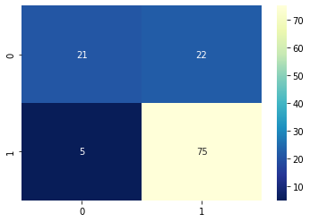
Classification Report
from sklearn.metrics import classification_report

print(classification_report(y_test, y_pred_test))
Variable(Feature) Importance
# variable importance
importance = pd.Series(model.feature_importances_, index=df1.columns[0:len(df1.columns)-1]).sort_values(ascending=False)

plt.figure(figsize=(12, 4))
sns.barplot(x=importance, y=importance.index)
plt.xlabel('Score')
plt.ylabel('Features(Predictors)')
plt.title("Feature Importance")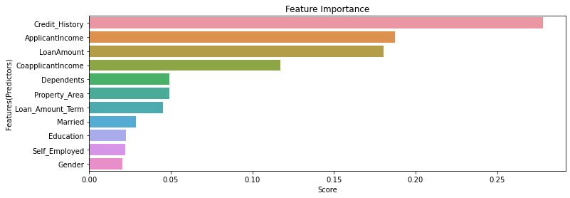
From the above graph, we can know that some variables(“Gender”, “Self_Employed”, “Education”) are not so important. Therefore, we can use by removing the features.