Table of Contents
- Definition
- Formulation
- Analysis Steps
- implementation of K-means Clustering
Definition
K-means clustering is an unsupervised machine learning method used to partition a set of observations into k clusters.
Unsupervised learning in artificial intelligence is a type of machine learning that learns from data without human supervision. Unlike supervised learning, unsupervised machine learning models are given unlabeled data and allowed to discover patterns and insights without any explicit guidance or instruction.
Formulation
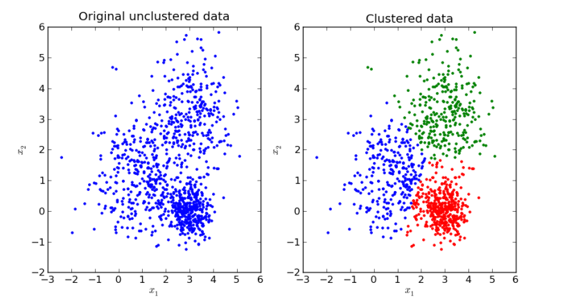
The key objective of a k-means algorithm is to organize data into clusters such that there is high intra-cluster similarity and low inter-cluster similarity. An item will only belong to one cluster, not several, that is, it generates a specific number of disjoint, nonhierarchical clusters.
K-means uses the strategy of divide and concur, and it is a classic example for an expectation maximization (EM) algorithm. K-Means is widely used for many applications:
- Image Segmentation
- Clustering Gene Segmentation Data
- News Article Clustering
- Clustering Languages
- Species Clustering
- Anomaly Detection
K-means Clustering Steps
If scales of features(predictor variables) are different, standardization is neccessary.
- Select K.
- Randomly select initial cluster seeds(centroids).
- Calculate distance from each object to each cluster seed(centroid).
We can use one of several distances: Euclidean distance, Square Euclidean distance, Manhattan distance, Chebyshev distance, Minkowski distance, Canberra distance, Chi square distance, Gower distance, User defined function for distance calculation between two points.
- Assign each object to the closest cluster.
- Compute the new centroid for each cluster.
- Iterate steps 3-5.
Stop condition: This is based on convergence criteria.
- No change in clusters
- Max iterations
K-means has problems when clusters are of differing sized, densities, and non globular shapes.
Distance for use of K-means Clustering
Euclidean Distance
$d\left( {a,\,b} \right) = \sqrt {\sum\limits_{i = 1}^p {{{\left( {{a_i} – {b_i}} \right)}^2}} } $
Where p is the number of dimensions (attributes), ${a_k}\,\,and\,\,{b_k}$ are, respectively, the k-th attributes(components) or data objects a and b.
Manhattan Distance
$d\left( {a,\,b} \right) = \sum\limits_{i = 1}^p {|{a_k} – {b_k}|} $
Minkowski Distance
Minkowski Distance is a generalization of Euclidean Distance.
$d\left( {a,\,b} \right) = {\left( {\sum\limits_{i = 1}^p {{{\left( {{a_k} – {b_k}} \right)}^m}} } \right)^{\frac{1}{m}}}$
Where r is a parameter, p is the number of dimensions (attributes) and ${a_k}\,\,and\,\,{b_k}$ are, respectively, the k-th attributes (components) or data objects a and b.
– $r = 1\,\,\,\,\,\, \Rightarrow \,\,\,\,{\bf{Manhattan}}(L_1 – norm)$ distance
– $r = 2\,\,\,\,\,\, \Rightarrow \,\,\,\,{\bf{Euclidean}}({L_2} – norm)$ distance
– $r = \infty \,\,\,\, \Rightarrow \,\,\,\,{\bf{supremum}}({L_{\max }} – norm,\,\,\,{L_\infty } – norm)$ distance
Finding Optimal K
To find optimal K, we can use the following methods.
- Elbow Method
The elbow method is a graphical method for finding the optimal K value in a k-means clustering algorithm. The elbow graph shows the within-cluster-sum-of-square (WCSS) values on the y-axis corresponding to the different values of K (on the x-axis).
$$\eqalign{
& {\bf{WCSS}} = \sum\limits_{i = 1}^K {\sum\limits_{x \in {C_i}} {{{\left( {x – {\mu _i}} \right)}^2}} } \cr
& \,\,\,\,\,\,\,where, \cr
& \,\,\,\,\,\,\,\,\,\,\,\,\,K\,:\,the\,\,number\,\,of\,\,clusters,\,\,{C_i}\,:\,{i^{th}}\,\,cluster,\,\,{\mu _i}\,:\,centroid\,\,of\,\,{i^{th}}\,\,cluster \cr} $$
Silhouette refers to a method of interpretation and validation of consistency within clusters of data.
The silhouette value is a measure of how similar an object is to its own cluster (cohesion) compared to other clusters (separation). The silhouette ranges from −1 to +1, where a high value indicates that the object is well matched to its own cluster and poorly matched to neighboring clusters.
$$\eqalign{
& {s_i} = \frac{{{b_i} – {a_i}}}{{\max \left\{ {{a_i},{b_i}} \right\}}} \cr
& \,\,\,\,\,where, \cr
& \,\,\,\,\,\,\,\,\,\,{a_i}:average\,\,distan ce\,\,between\,\,i\,\,and\,\,all\,\,of\,\,the\,\,other\,\,points\,\,in\,\,{\bf{its}}\,\,{\bf{own}}\,\,{\bf{cluster}} \cr
& \,\,\,\,\,\,\,\,\,{b_i}:distance\,\,between\,\,i\,\,and\,\,its\,\,next\,\,nearest\,\,cluster\,\,centroid \cr} $$
Analysis Steps
Here are the key steps to understand a our model:
- Data Collection: Gather the dataset containing the relevant information we want to model.
- Data Visualization and Data preprocessing:
- Data cleaning: Check for missing values and outliers.Handle them appropriately by imputing missing data or removing outliers
- Feature Selection/Engineering: Determine which independent variable are relevant for our model. we might need to transform or engineer features to make them suitable for regresion
Implementation of K-means Clustering
Problem Statement
There is data of customers that use credit card for last 6 months.
Here, we are going to classify customers using K-means clustering analysis.
Data
The data contains the following features in excel file format:
- CUST_ID : Identification of Credit Card holder (Categorical)
- BALANCE : Balance amount left in their account to make purchases (
- BALANCE_FREQUENCY : How frequently the Balance is updated, score between 0 and 1 (1 = frequently updated, 0 = not frequently updated)
- PURCHASES : Amount of purchases made from account
- ONEOFF_PURCHASES : Maximum purchase amount done in one-go
- INSTALLMENTS_PURCHASES : Amount of purchase done in installment
- CASH_ADVANCE : Cash in advance given by the user
- PURCHASES_FREQUENCY : How frequently the Purchases are being made, score between 0 and 1 (1 = frequently purchased, 0 = not frequently purchased)
- ONEOFFPURCHASESFREQUENCY : How frequently Purchases are happening in one-go (1 = frequently purchased, 0 = not frequently purchased)
- PURCHASESINSTALLMENTSFREQUENCY : How frequently purchases in installments are being done (1 = frequently done, 0 = not frequently done)
- CASHADVANCEFREQUENCY : How frequently the cash in advance being paid
- CASHADVANCETRX : Number of Transactions made with “Cash in Advanced”
- PURCHASES_TRX : Numbe of purchase transactions made
- CREDIT_LIMIT : Limit of Credit Card for user
- PAYMENTS : Amount of Payment done by user
- MINIMUM_PAYMENTS : Minimum amount of payments made by user
- PRCFULLPAYMENT : Percent of full payment paid by user
- TENURE : Tenure of credit card service for user
Import Necessary Libraries
NumPy is a Python library used for working with arrays. It also has functions for working in domain of linear algebra, fourier transform, and matrices. NumPy can be used to perform a wide variety of mathematical operations on arrays. It adds powerful data structures to Python that guarantee efficient calculations with arrays and matrices and it supplies an enormous library of high-level mathematical functions that operate on these arrays and matrices.
Pandas is a Python library used for working with data sets. It has functions for analyzing, cleaning, exploring, and manipulating data. Pandas is a fast, powerful, flexible and easy to use open source data analysis and manipulation tool, built on top of the Python programming language.
Matplotlib is a comprehensive library for creating static, animated, and interactive visualizations in Python. Matplotlib makes easy things easy and hard things possible. Create publication quality plots. Make interactive figures that can zoom, pan, update. Customize visual style and layout.
Seaborn is a Python data visualization library based on matplotlib. It provides a high-level interface for drawing attractive and informative statistical graphics. It builds on top of matplotlib and integrates closely with pandas data structures. Seaborn helps we explore and understand our data.
Scikit-learn is probably the most useful library for machine learning in Python. The sklearn library contains a lot of efficient tools for machine learning and statistical modeling including classification, regression, clustering and dimensionality reduction.
pyclustering is an open source Python, C++ data-mining library under BSD-3-Clause License. The library provides tools for cluster analysis, data visualization and contains oscillatory network models. pyclustering provides Python and C++ implementation almost for each algorithm, method, etc.
This library allows us to implement K-means clustering algorithm using another distances Not Euclidean distance.
# Supress Warnings
import warnings
warnings.filterwarnings('ignore')

# import the numpy and pandas packages
import numpy as np
import pandas as pd

# to visualize data
import matplotlib.pyplot as plt
import seaborn as sns

# to split arrays or matrices into random train and test subsets
from sklearn.model_selection import train_test_split
from sklearn.metrics import accuracy_score
from sklearn.model_selection import cross_val_score, KFold

# to import K-means clustering model from sklearn package
from sklearn.cluster import KMeans
from sklearn.metrics import silhouette_score

# to import K-means clustering model from pyclustering package
!pip3 install pyclustering
from pyclustering.cluster.kmeans import kmeans as pykmeans, kmeans_visualizer
from pyclustering.cluster.center_initializer import kmeans_plusplus_initializer
from pyclustering.utils.metric import distance_metric, type_metric
from pyclustering.cluster.encoder import cluster_encoder

# import category encoders
# !pip install category_encoders
import category_encoders as ce
from sklearn.preprocessing import StandardScaler, normalize
Data Collection
# data source
url = "./K-meansClustering_data.csv"
# reading data
df = pd.read_csv(url)
df.head()
row_cnt0 = df.shape[0]
print("The number of rows : %d.\nThe number of columns is : %d." % (row_cnt0, df.shape[1]))
The number of rows: 8950
The number of columns is: 18
# data information
df.info()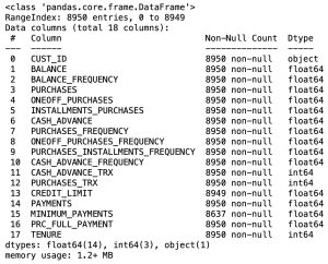
Data Processing
- Removing the unneccesary variables
- Removing null values
- Removing the duplicated values
# Removing the unneccesary variables because id variable doesn't affect diagnosis.
df_o = df.copy()
df = df.drop('CUST_ID', axis=1)
df
# Checking missing values
df.isnull().sum()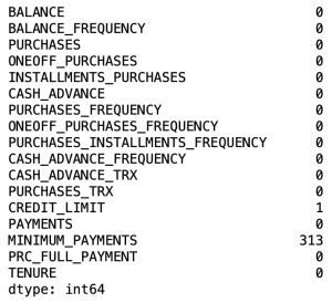
# Removing Null values
df = df.dropna(how='any',axis=0)
df_o = df_o.dropna(how='any',axis=0)
row_cnt1 = df.shape[0]
print("The number of rows deleted : %d" % (row_cnt0 - row_cnt1))
The number of rows deleted: 314
There are many missing values in our dataset.
# Checking for the presence of duplicate values. If there exists, we have to remove the rows.
df = df.drop_duplicates()
print("The number of rows removed: %d." % (row_cnt1 - df.shape[0]))
The number of rows removed: 0
There are no the duplicated values.
Correlation Analysis of Variables
# Evaluating correlation of variables to prevent overfitting
plt.figure(figsize=(16, 16))
sns.heatmap(df.corr(),annot=True, cmap='BrBG_r')
plt.show()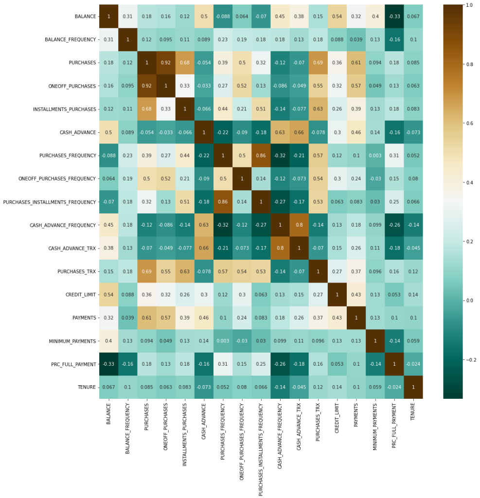
There is one considerable coefficient of correlation larger than 0.9. We need to remove some variables based on correlation analysis.
# Removing of some variables
df1 = df.drop('ONEOFF_PURCHASES', axis=1)
df1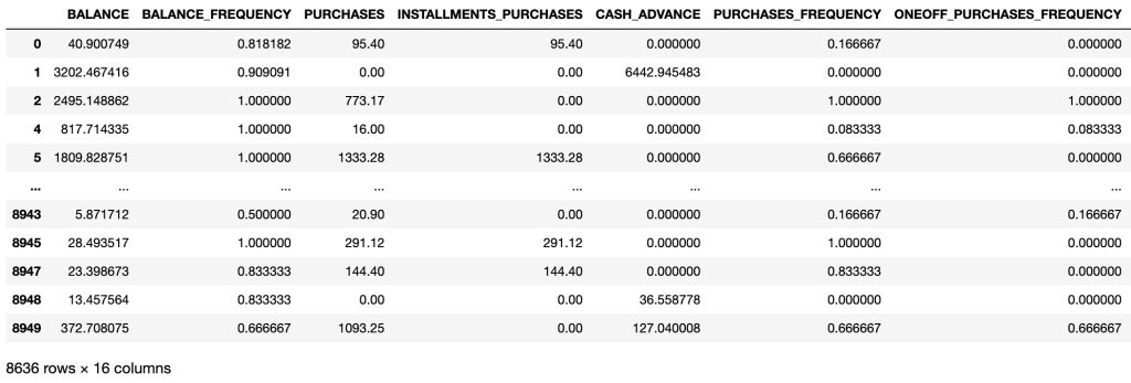
Visualizing of Data
# we can see each relationship between variables.
plt.figure(figsize=(16, 16))
sns.pairplot(df1)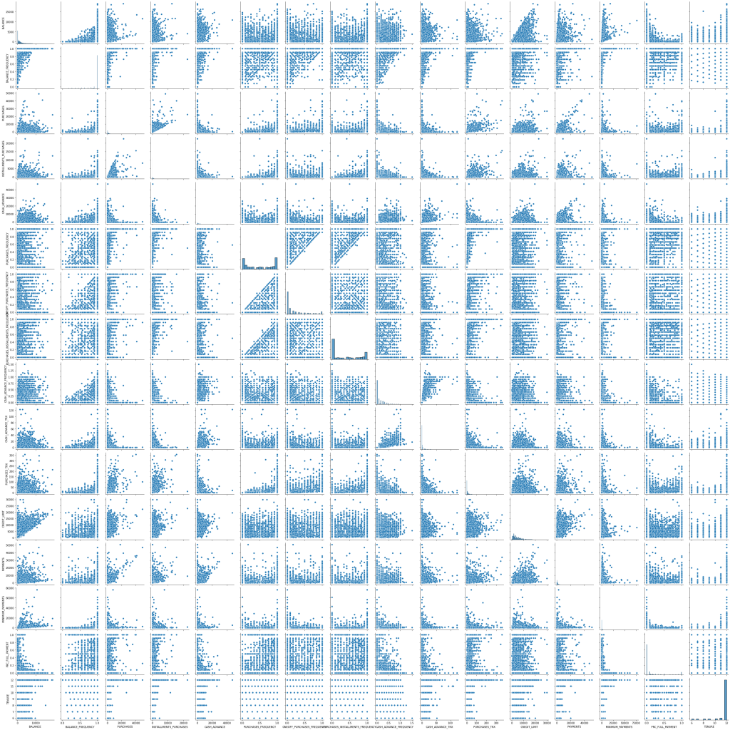
Standardization
Standardization is very necessary, if scales differ. Because it can not be calculated with different scales.
# Showing minimuns and maximums for each variable to scale
pd.DataFrame({'Min':np.min(df1), 'Max':np.max(df1)})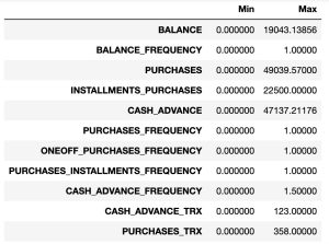
From the above table, we can know that scales are different. Therefore, we have to standardize predictor variables.
StandardScaler function in sklearn.preprocessing uses the following formula to standardize:
$\eqalign{
& {\bf{standardization}} \cr
& \,\,\,\,\,\,\,\,\,\,\,\,\,\,\,z = \frac{{x – \mu }}{\sigma } \cr
& where, \cr
& \,\,\,\,\,\,\,\,\,\,\,\,\,{\bf{mean}}:\,\,\mu = \frac{1}{N}\sum\limits_{i = 1}^n {{x_i}} ,\,\,\,\,\,\,\,\,\,{\bf{standard}}\,\,{\bf{deviation}}\,\,\,\sigma = \sqrt {\frac{1}{N}\sum\limits_{i = 1}^n {{{\left( {{x_i} – \mu } \right)}^2}} } \cr} $
$\eqalign{
& {\bf{normalize:}} \cr
& \,\,\,\,\,\,\,\,\,\,\,\,\,\,can\,\,be\,\,normalized\,\,using\,\,one\,\,of\,{L_1} – norm,\,\,\,{L_2} – norm\,\,and\,\,\,{L_{\max }} – norm \cr} $
# Standardizing and normalizing input(independent) variables
scaler = StandardScaler()
df2 = pd.DataFrame(normalize(scaler.fit_transform(df1)))
df2
Building K-means Clustering and Finding optimal K Using Sklearn
# Finding optimal k by Elbow Method

# within-cluster sum of squares
wcss = []

k_range = range(1, 30)
for k in k_range:
    kmeans = KMeans(n_clusters=k, max_iter=300).fit(df2)
    wcss.append(kmeans.inertia_ ) # Sum of squared distances of samples to their closest cluster center

plt.figure(figsize=(16, 6))
plt.plot(k_range, wcss, 'r-o')
plt.xlabel('k')
plt.ylabel("wcss")
plt.title('WCSS vs. the number of clusters, k(Elbow Method)')
plt.show()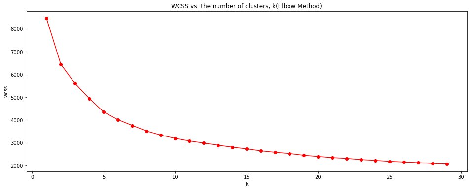
When the number of clusters, k increases, WCSS value rapidly decreases at the beginning and then decreases slowly after k = 8. Therefore, we can set the optimal K as 8 by Elbow Method.
# Finding optimal k by Silhouette Method
k_range = range(2, 30)

sc = [] # Silhouette Coefficient

for k in k_range:
    sc.append(silhouette_score(df2, KMeans(n_clusters = k, max_iter=300).fit_predict(df2)))

plt.figure(figsize=(16, 6))
plt.bar(k_range, sc)
plt.xlabel('k')
plt.ylabel("Silhouette Coefficient")
plt.title('Silhouette Coefficient vs. the number of clusters, k(Silhouette Method)')
plt.show()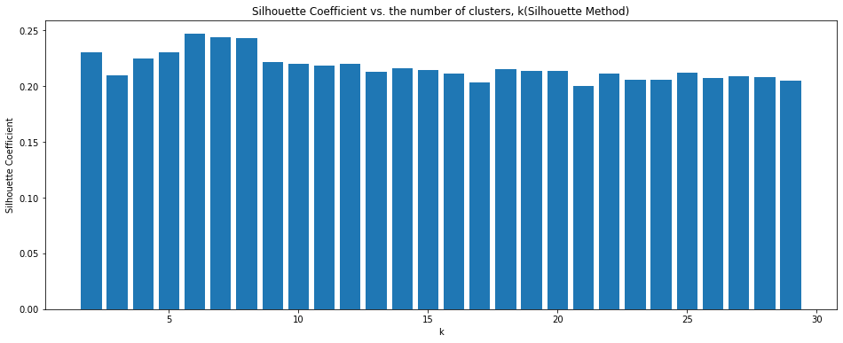
We can know that Silhouette Coefficient is relatively high when the number of clusters, k is between 6-8. We can set the optimal K as 6(the highest value)
From our analysis, it is better to set the optimal K as 8
# K-means Clusering
kmeans = KMeans(n_clusters=8, max_iter=300).fit(df2)
cluster_info = kmeans.labels_pd.DataFrame({'Customer ID':df_o['CUST_ID'], 'cluster number':cluster_info})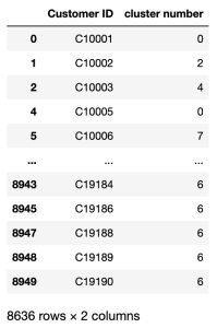
Building K-means Clustering and Finding optimal K using pyclustering package
Here, we are going to use MANHATTAN distance(${L_1} – norm$).
# Finding optimal k by Elbow Method

# within-cluster sum of squares
wcss = []

# create metric that will be used for clustering using MANHATTAN distance
metric = distance_metric(type_metric.MANHATTAN)

# k range
k_range = range(1, 30)

for k in k_range:
    # Prepare initial centers using K-Means++ method.
    initial_centers = kmeans_plusplus_initializer(df2, k).initialize()

    # create instance of K-Means using specific distance metric:
    kmeans_instance = pykmeans(df2, initial_centers, metric=metric)

    kmeans_instance.process()
    # cluster analysis results - clusters and centers
    clusters = kmeans_instance.get_clusters()
    centers = kmeans_instance.get_centers()

    # enumerate encoding type to index labeling to get labels
    encoding = kmeans_instance.get_cluster_encoding()
    encoder = cluster_encoder(encoding, clusters, df2)
    labels = encoder.set_encoding(0).get_clusters()

    ssd = 0 # saving sum of squared distances
    for i in range(len(labels)):
        ssd = ssd + metric(df2.iloc[i], centers[labels[i]])**2
    wcss.append(ssd)

plt.figure(figsize=(16, 6))
plt.plot(k_range, wcss, 'c--o')
plt.xlabel('k')
plt.ylabel("wcss")
plt.title('WCSS vs. the number of clusters, k(Elbow Method)')
plt.show()
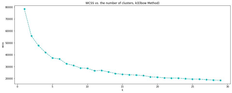
WCSS graphs using EUCLIDEAN distance(in sklearn package) and MANHATTAN distance(in pyclustering package) are very similar. Therefore, we can choose the optimal K a 8.
Leave a Reply