Table of Contents
- Definition
- Types of KNN(K-nearest neighbors)
- Formulation
- Analysis Steps
- Classification problem Using KNN
Definition
KNN(K-nearest neighbors algorithm is a non-parametric supervised learning for classification and regression.
Types of KNN(K-nearest neighbors)
- KNN regression approximates the association between independent variables and the continuous outcome by averaging the observations in the same neighbourhood and calculates the average or weighted average of the target values of the K neighbors to predict the value for the input data point.
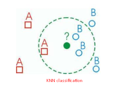
- KNN classification classifies by “MAJORITY VOTES” for K neighbor classes, assigning to the most common class among its K nearest neighbors (by measuring “distant” between data).
Formulation
Feature of KNN
- Simple
- Classifies based on a similarity measure
- Non-parametric method
KNN is non-parametric since it makes no assumptions about the data it is analyzing, i.e. the model is distributed from the data. - It does not “learn” until the test example is given.
Whenever we have a new data to classify, we find its K-nearest neighbors from the training data.
KNN Steps
- Determine parameter K = the number of nearest neighbors
- Calculate the distance between the new data point(query-instance) and all the training examples
- Sort the distance and determine nearest neighbors based on the k-th minimum distance
- Gather the values of target variable for the K nearest neighbors
- Use simple majority of the category of nearest neighbors as the prediction value of the query instance
Decision Boundary
Voronoi Diagram
- Describes the areas that are nearest to any given point, given a set of data.
- Each line segment is equidistant between two points of opposite class
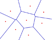
With large number of examples and possible noise in the labels, the decision boundary can become nasty.
Effect of K
Larger k produces smoother boundary effect
When K==N, always predict the majority class
Understanding of Similarity and Dissimilarity
Similarity
- Numerical measure of how alike two data objects are.
- Is higher when objects are more alike.
- Often falls in the range [0,1][0,1]
Dissimilarity
- Numerical measure of how different are two data objects
- Lower when objects are more alike
- Minimum dissimilarity is often 0
- Upper limit varies
Proximity refers to a similarity or dissimilarity
Distance and Similarity for use of KNN
Euclidean Distance
$d\left( {a,\,b} \right) = \sqrt {\sum\limits_{i = 1}^p {{{\left( {{a_i} – {b_i}} \right)}^2}} } $
Where p is the number of dimensions (attributes), ${a_k}\,\,and\,\,{b_k}$ are, respectively, the k-th attributes(components) or data objects a and b.
Standardization is necessary, if scales differ.
$d\left( {a,\,b} \right) = \sqrt {\sum\limits_{i = 1}^p {{{\left( {{a_i} – {b_i}} \right)}^2}} } $
Manhattan Distance
$d\left( {a,\,b} \right) = \sum\limits_{i = 1}^p {|{a_k} – {b_k}|} $
Minkowski Distance
Minkowski Distance is a generalization of Euclidean Distance.
$d\left( {a,\,b} \right) = {\left( {\sum\limits_{i = 1}^p {{{\left( {{a_k} – {b_k}} \right)}^m}} } \right)^{\frac{1}{m}}}$
Where r is a parameter, p is the number of dimensions (attributes) and ${a_k}\,\,and\,\,{b_k}$ are, respectively, the k-th attributes (components) or data objects a and b.
– $r = 1\,\,\,\,\,\, \Rightarrow \,\,\,\,{\bf{Manhattan}}(L_1 – norm)$ distance
– $r = 2\,\,\,\,\,\, \Rightarrow \,\,\,\,{\bf{Euclidean}}({L_2} – norm)$ distance
– $r = \infty \,\,\,\, \Rightarrow \,\,\,\,{\bf{supremum}}({L_{\max }} – norm,\,\,\,{L_\infty } – norm)$ distance
Cosine Similarity
Cosine similarity measures the similarity between two vectors of an inner product space. It is measured by the cosine of the angle between two vectors and determines whether two vectors are pointing in roughly the same direction. It is often used to measure document similarity in text analysis.
If 𝑑1 and 𝑑2 are two document vectors
$\cos \left( {{{\bf{d}}_1},\,\,{{\bf{d}}_2}} \right) = \frac{{{{\bf{d}}_1} \cdot {{\bf{d}}_2}}}{{\left\| {{{\bf{d}}_1}} \right\|\,\,\left\| {{{\bf{d}}_2}} \right\|}}$
$\cos \left( {{{\mathbf{d}}_1},\,\,{{\mathbf{d}}_2}} \right) = \left\{ \begin{gathered}
\;\;\;1:\,\,\,\,exactly\,the\,\,same\;\;\\
0:\,\,\,\,orthogonal \;\;\;\;\;\;\;\;\\
– 1:\,\,\,exactly\,opposite\;\;\;\\
\end{gathered} \right.$
Analysis Steps
Here are the key steps to understand a our model:
- Data Collection: Gather the dataset containing the relevant information we want to model.
- Data Visualization and Data preprocessing:
- Data cleaning: Check for missing values and outliers.Handle them appropriately by imputing missing data or removing outliers
- Feature Selection/Engineering: Determine which independent variable are relevant for our model. we might need to transform or engineer features to make them suitable for regresion
- Assumption Check: If the given assumptions is not satisfied, we may need to apply transformations or consider different modeling techniques.
- Split Data: Divide our dataset into a training set and testing set. The training set is used to train the model and the testing set is sued to evaluate its preformance.
There are several methods for spliting datasets for machine learning and data analysis, Each method serves different purpose and has its advantages and disadvantages. Here are some comon dataset splitting methods along with step by step explanations for each:- Train-test Split(Holdout Method) – purpose to create two seperate sets, one for training and one for testing the mocel
Steps:- Randomly shuffle the dataset to ensure teh data is well distributed.
- Split the data into two parts, typically with a ratio like 70-30 or 80-20, where one part is for training and the other for testing
- Train our machine learning model on the training set
- Evaluate the model performance on the test set
K-Fold Cross Validation: Purpose to assess the model’s performance by training and testing it on different subsets of the data. steps: A. Divide the dataset into K equal sized folds B. For each fold(1 to K) treat it as a test set and the remaining K-1 folds as the training set. C. Train and evaluate the model on each of the K iterations. D. Calculate performance metrics(accuracy) by averaging the results from all iterations.
startified Sampling: purpose to ensure that the proportion of different classes in the dataset is maintained in teh train and test sets steps: A. Identify the target variable B. Stratify the data by the target variable to create representative subsets. C. perform a train_test split on these stratified subsets to maintain class balance in both sets
Time series split: purpose for time series data where the order of data oints matter steps A. sort the dataset based on the time or date variable B. Divide the data into training and testing sets such that the training set consists of past data and the testing set contains future data. - Leave one out cross validation – Purpose to leave out a single data point as the test set in each iteration. Steps: For each data point in the dataset, create a training set with all other data points. Train and test the model for each data point separately. Calculate the performance metrics based on the predictions from each iteration.
Group k-fold cross validation:purpose to accouont for groups or slusters in the data
Steps:- Randomly sample data points with replacement to create multiple bootstrap samples.
- Train and evaluate the model on each bootstrap sample.
- Calculate performance metrics based on the results of each sample.
- Train-test Split(Holdout Method) – purpose to create two seperate sets, one for training and one for testing the mocel
- Model Building:
- Choose the model: select either 3 types of models according to the values of dependent variable: binomial or multinomial, ordinal
- Fit the model: use the training data to estimate the coefficients that maximizes the likelihood of observing the data given
- Model Evaluation:
If our problem is Regression problem, use appropiate metrics like Mean Squared Error(MSE), Root Mean Squared Error(RMSE) or R-squared to evaluate how well our model fits.
If our problem is Classification problem, use appropiate metrics like acuracy, precision, recall, f1 Score, AUC-ROC or AUC-PR to evaluate how well our model fits.
Classification problem Using KNN
Problem Statement
A cancer diagnosis can affect the emotional health of patients, families, and caregivers. Common feelings during this life-changing experience include anxiety, distress, and depression.
Here, we are going to predict the type of cancer diagnosis using KNN.
Cancer diagnosis has two type of values:
- M = malignant
- B = benign
Also, we are going to extract good k value based on error rate.
Data
The data contains the following features in excel file format:
- id
- diagnosis
- radius_mean
- texture_mean
- perimeter_mean
- area_mean
- smoothness_mean
- compactness_mean
- concavity_mean
- concave points_mean
- symmetry_mean
- fractal_dimension_mean
- radius_se
- texture_se
- perimeter_se
- area_se
- smoothness_se
- compactness_se
- concavity_se
- concave points_se
- symmetry_se
- fractal_dimension_se
- radius_worst
- texture_worst
- perimeter_worst
- area_worst
- smoothness_worst
- compactness_worst
- concavity_worst
- concave points_worst
- symmetry_worst
- fractal_dimension_worst
Import Necessary Libraries
NumPy is a Python library used for working with arrays. It also has functions for working in domain of linear algebra, fourier transform, and matrices. NumPy can be used to perform a wide variety of mathematical operations on arrays. It adds powerful data structures to Python that guarantee efficient calculations with arrays and matrices and it supplies an enormous library of high-level mathematical functions that operate on these arrays and matrices.
Pandas is a Python library used for working with data sets. It has functions for analyzing, cleaning, exploring, and manipulating data. Pandas is a fast, powerful, flexible and easy to use open source data analysis and manipulation tool, built on top of the Python programming language.
Matplotlib is a comprehensive library for creating static, animated, and interactive visualizations in Python. Matplotlib makes easy things easy and hard things possible. Create publication quality plots. Make interactive figures that can zoom, pan, update. Customize visual style and layout.
Seaborn is a Python data visualization library based on matplotlib. It provides a high-level interface for drawing attractive and informative statistical graphics. It builds on top of matplotlib and integrates closely with pandas data structures. Seaborn helps we explore and understand our data.
Scikit-learn is probably the most useful library for machine learning in Python. The sklearn library contains a lot of efficient tools for machine learning and statistical modeling including classification, regression, clustering and dimensionality reduction.
# Supress Warnings
import warnings
warnings.filterwarnings('ignore')

# import the numpy and pandas packages
import numpy as np
import pandas as pd

# to visualize data
import matplotlib.pyplot as plt
import seaborn as sns

# to split arrays or matrices into random train and test subsets
from sklearn.model_selection import train_test_split
from sklearn.metrics import accuracy_score
from sklearn.model_selection import cross_val_score, KFold

# to import KNN Classifier model
from sklearn.neighbors import KNeighborsClassifier

# import category encoders
# !pip install category_encoders
import category_encoders as ce
from sklearn.preprocessing import StandardScaler
Data Collection
# data source
url = "./KNN_cancer.csv"
# reading data
df = pd.read_csv(url)
df.head()
row_cnt0 = df.shape[0]
print("The number of rows : %d.\nThe number of columns is : %d." % (row_cnt0, df.shape[1]))
The number of rows: 569
The number of columns is: 32
# data information
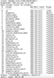
df.info()
In the Pandas library, the info() method prints summary information about the DataFrame.
Data Processing
- Removing the unneccesary variables
- Removing null values
- Removing the duplicated values
# Removing the unneccesary variables because id variable doesn't affect diagnosis.
df = df.drop('id', axis=1)
df
# Checking missing values
df.isnull().sum()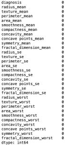
# Removing Null values
df = df.dropna(how='any',axis=0)
row_cnt1 = df.shape[0]
print("The number of rows deleted : %d" % (row_cnt0 - row_cnt1))
The number of rows deleted: 0
There are no missing values in our dataset.
# Checking for the presence of duplicate values. If there exists, we have to remove the rows.
df = df.drop_duplicates()
print("The number of rows removed: %d." % (row_cnt1 - df.shape[0]))
The number of rows removed: 0
There are no the duplicated values.
# Independent variable and dependent variable
X = df.drop('diagnosis', axis=1)
y = df['diagnosis']
X
Converting string variables into numerical variables
All the calculations are performed only with numbers. Thus, we need to convert the useful features into numbers.
# Converting Target variable values into numbers
unique_val = y.unique()
y = y.replace((unique_val),(1,0))
y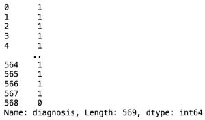
Correlation Analysis of independent Variables
# Evaluating correlation of variables to prevent overfitting
plt.figure(figsize=(16, 16))
sns.heatmap(X.corr(),annot=True, cmap='BrBG_r')
plt.show()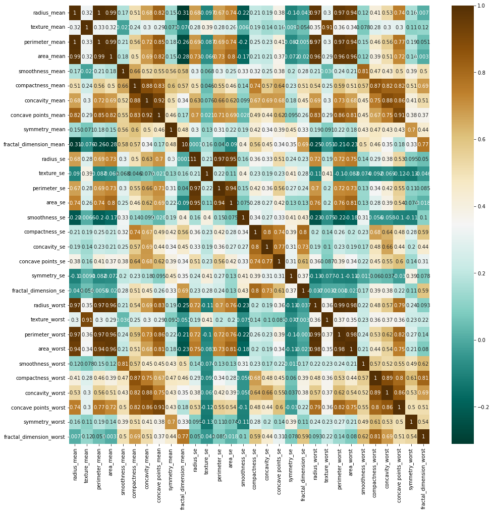
There are many considerable coefficients of correlation larger than 0.9. We need to remove some variables based on correlation analysis.
# Removing of some variables(10 variables)
X = X.drop('concave points_worst', axis=1)
X = X.drop('area_worst', axis=1)
X = X.drop('perimeter_worst', axis=1)
X = X.drop('texture_worst', axis=1)
X = X.drop('radius_worst', axis=1)
X = X.drop('area_se', axis=1)
X = X.drop('perimeter_se', axis=1)
X = X.drop('perimeter_mean', axis=1)
X = X.drop('area_mean', axis=1)
X = X.drop('concave points_mean', axis=1)

# Correlation analysis
plt.figure(figsize=(16, 16))
sns.heatmap(X.corr(),annot=True, cmap='BrBG_r')
plt.show()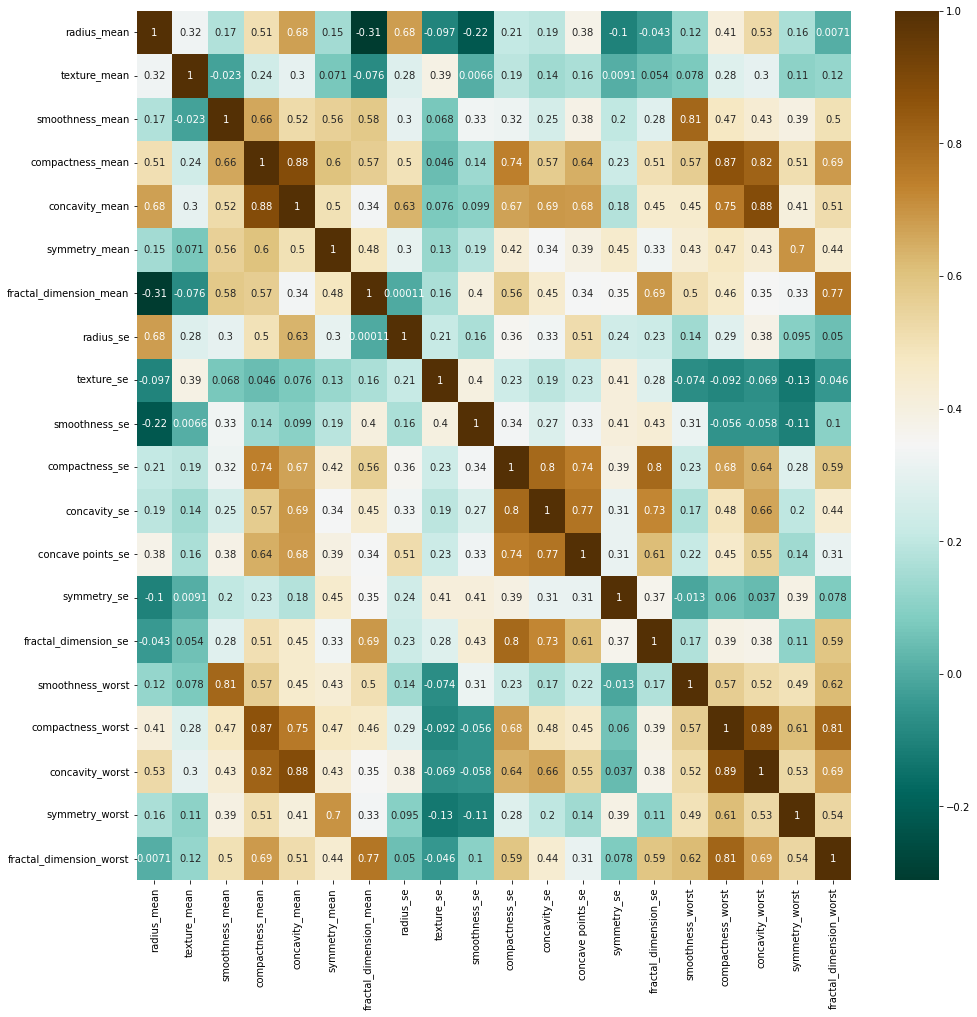
Visualizing of Data
# Visualizing frequency of target variable
plt.figure(figsize=(8, 6))
ax = sns.countplot(x='diagnosis', data=df)
for container in ax.containers:
    ax.bar_label(container)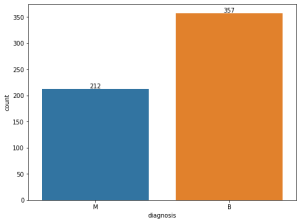
# we can see each relationship between variables.
sns.pairplot(X)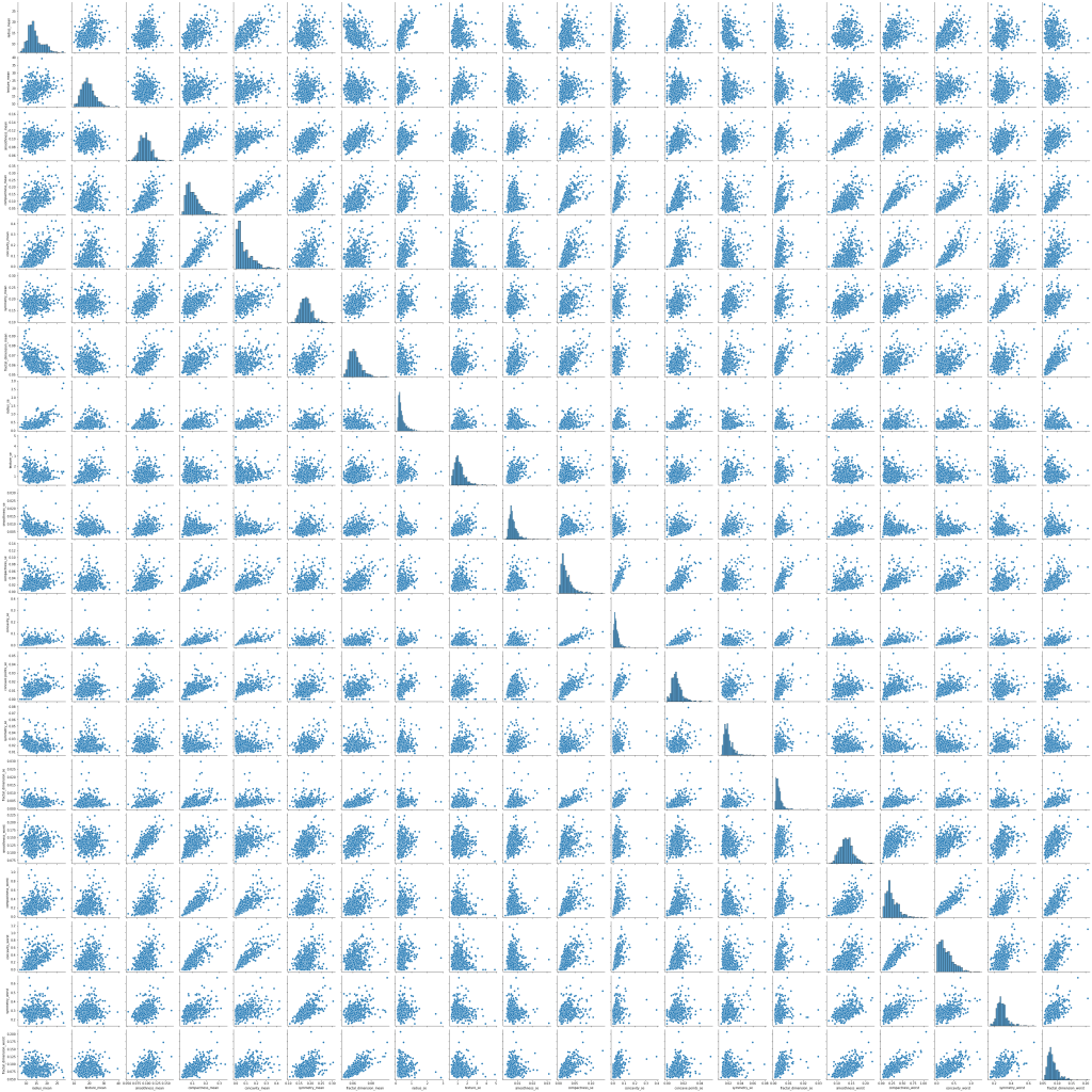
Train-Test Split
# data split
X_train, X_test, y_train, y_test = train_test_split(X, y, train_size = 0.8, test_size = 0.2, random_state = 50)
X_train
y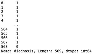
Standardization
In KNN, standardization is very necessary, if scales differ. Because it can not be calculated with different scales.
# Showing minimuns and maximums for each variable to scale
pd.DataFrame({'Min':np.min(X), 'Max':np.max(X)})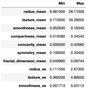
From the above table, we can know that scales are different. Therefore, we have to standardize predictor variables.
StandardScaler function in sklearn.preprocessing uses the following formula to standardize:
$\eqalign{
& {\bf{standardization}} \cr
& \,\,\,\,\,\,\,\,\,\,\,\,\,\,\,z = \frac{{x – \mu }}{\sigma } \cr
& where, \cr
& \,\,\,\,\,\,\,\,\,\,\,\,\,{\bf{mean}}:\,\,\mu = \frac{1}{N}\sum\limits_{i = 1}^n {{x_i}} ,\,\,\,\,\,\,\,\,\,{\bf{standard}}\,\,{\bf{deviation}}\,\,\,\sigma = \sqrt {\frac{1}{N}\sum\limits_{i = 1}^n {{{\left( {{x_i} – \mu } \right)}^2}} } \cr} $
# Standardizing input(independent) variables
scaler = StandardScaler()
scaler.fit(X_train)

X_train_standardized = scaler.transform(X_train)
X_train_standardized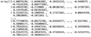
Building Naive Bayes Classification Model
Because the predictors take up a discrete value, we can use multinomial naive bayes classifier model.
# Creating instance of model
model = KNeighborsClassifier(n_neighbors=20)

# Fitting train data
model.fit(X_train_standardized, y_train)
# Predicting based on train data
y_pred_train = model.predict(X_train_standardized)Now X_test has to be standardized based on the existing scaler instance(with $\mu ,\,\sigma $).
# Standardizing X_test
X_test_standardized = scaler.transform(X_test)

# Predicting based on test data
y_pred_test = model.predict(X_test_standardized)
X_test_standardized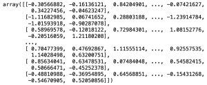
Model Evaluation
Comparison of accuracies for train and test datasets
print('accuracy score for train dataset: %f.3' % accuracy_score(y_train, y_pred_train))
print('accuracy score for test dataset: %f.3' % accuracy_score(y_test, y_pred_test))
accuracy score for train dataset: 0.945055.3
accuracy score for test dataset: 0.964912.3
Confusion Matrix
A confusion matrix is a performance evaluation tool in machine learning, representing the accuracy of a classification model. It displays the number of true positives, true negatives, false positives, and false negatives.
- True positives (TP) occur when the model accurately predicts a positive data point.
- True negatives (TN) occur when the model accurately predicts a negative data point.
- False positives (FP) occur when the model predicts a positive data point incorrectly.
- False negatives (FN) occur when the model mispredicts a negative data point.
# confusion matrix
from sklearn.metrics import confusion_matrix

confusion_m = confusion_matrix(y_test, y_pred_test)sns.heatmap(confusion_m, annot=True, fmt='d', cmap='YlGnBu_r')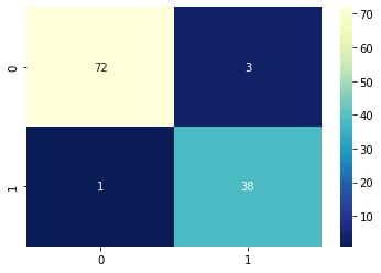
Classification Report
from sklearn.metrics import classification_report

print(classification_report(y_test, y_pred_test))
Choosing the best K
Now we don’t know the optimal K value. Thus, it needs to obtain the best K.
err_rate_train = []
err_rate_test = []
max_K = 100
K_range = np.array(range(1, max_K))

for K in K_range:
    # Creating instance of model
    model = KNeighborsClassifier(n_neighbors=K)

    # Fitting train data
    model.fit(X_train_standardized, y_train)

    # Predicting based on train and test data
    y_pred_train = model.predict(X_train_standardized)
    y_pred_test = model.predict(X_test_standardized)

    # Error rate
    err_rate_train.append(1 - accuracy_score(y_train, y_pred_train))
    err_rate_test.append(1 - accuracy_score(y_test, y_pred_test))


# Plotting Error rate vs. K
plt.figure(figsize=(16, 6))
plt.plot(K_range, err_rate_train, "ro-")
plt.plot(K_range, err_rate_test, "go-")
plt.legend(["error rate for train", "error rate for test"])
plt.show()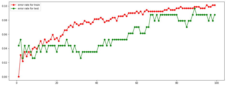
We are going to select the largest K of K values that error rate is less than 5% for both train and test dataset.
From the above graph, when K value increases, error rate increases, too.
Increasing speed of error rate is slow.
# Finding the best K
best_K = max(K_range[(np.array(err_rate_train) < 0.05) & (np.array(err_rate_test) < 0.05)])
best_K
Therefore, the optimal K value is 15