Naive Bayes Classifier

Table of Contents

• Definition
• Assumptions
• Types of Naive Bayes Classifier(Model)
• Formulation
• Analysis Steps
• Classification problem Using Naive Bayes Model

Definition

Naive Bayes classifier is a family of linear “probabilistic classifiers” which assumes that the features are conditionally independent, given the target class. The strength (naivety) of this assumption is what gives the classifier its name. These classifiers are among the simplest Bayesian network models.

Naive Bayes classifiers are highly scalable, requiring a number of parameters linear in the number of variables (features/predictors) in a learning problem. Maximum-likelihood training can be done by evaluating a closed-form expression, which takes linear time, rather than by expensive iterative approximation as used for many other types of classifiers.

The thought behind naive Bayes classification is to try to classify the data by maximizing P(O|Ci)P(Ci) using Bayes theorem of posterior probability (where O is the Object or tuple in a dataset and “i” is an index of the class). Naïve Bayes is part of a family of generative learning algorithms, meaning that it seeks to model the distribution of inputs of a given class or category. Unlike discriminative classifiers, like logistic regression, it does not learn which features are most important to differentiate between classes.

The Naïve Bayes classifier is a supervised machine learning algorithm that is used for classification tasks such as text classification.

Assumptions

• The naive Bayes classifier assumes that all features in the input data are independent of each other, which is often not true in real-world problem. This assumption significantly reduces the complexity of the calculations of the objective functions in terms of posterior probabilities.
• All features contribute equally to the outcome.

Types of Naive Bayes Classifier(Model)

There are different Naive Bayes classifiers:

• Gaussian Naive Bayes: When the predictors take up a continuous value and are not discrete, we assume that these values are sampled from a gaussian distribution.
• Multinomial Naive Bayes: The multinomial Naive Bayes classifier is suitable for classification with discrete features (e.g., word counts for text classification). The multinomial distribution normally requires integer feature counts. The features/predictors used by the classifier are the frequency of the words present in the document.
• Bernoulli Naive Bayes: This is similar to the multinomial naive bayes but the predictors are boolean variables. The parameters that we use to predict the class variable take up only values yes or no, for example if a word occurs in the text or not.
• Complement Naive Bayes: Complement Naive Bayes (CNB) is an adaptation of the standard Multinomial Naive Bayes (MNB) algorithm that is particularly suited for imbalanced data sets. Specifically, CNB uses statistics from the complement of each class to compute the model weights.
• Categorical Naive Bayes: The categorical Naive Bayes classifier is suitable for classification with discrete features that are categorically distributed. The categories of each feature are drawn from a categorical distribution.
• Out-of-core naive Bayes model fitting: This classifier is used to handle cases of large scale classification problems for which the complete training dataset might not fit in the memory.

Formulation

Let’s be the vector of random variables: ${\bf{x}} = ({x_1},{x_2}, \cdot \cdot \cdot ,{x_n})$

Understanding of Probabilistic Classification

In machine learning, a probabilistic classifier is a classifier that is able to predict, given an observation of an input, a probability distribution over a set of classes, rather than only outputting the most likely class that the observation should belong to. Probabilistic classifiers provide classification that can be useful in its own right or when combining classifiers into ensembles.

Methods to create classifiers

1) Medhod to model a classification rule directly
2) Method to model the probability of class memberships given input data
3) Method to make a probabilistic model of data within each class(Naïve Bayes is a example of a family of generative classification)
  

Here, 1) and 2) are cases of discriminative classification, 3) is a case of generative classification, 2) and 3) are cases of probabilistic classification

Comparison between Generative and Discriminative Classifiers

A deterministic model makes predictions based on a set of predefined rules and input data. The output is always the same if the same inputs are provided. In contrast, a generative model creates new data that is similar to a given dataset. The output can vary every time the model is run because it’s generating new data. The main difference between the two types of models is that deterministic models predict outcomes based on existing data, while generative models create new data.

Training classifiers involves estimating $f:{\text{ }}X \to Y,{\text{ }}or{\text{ }}P\left( {Y|X} \right)$

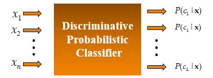
Discriminative Classifiers

Discriminative Classifiers learn what the features in the input are most useful to distinguish between the various possible classes.

– Assume some functional form for $P\left( {Y|X} \right)$
– Estimate parameters of $P\left( {Y|X} \right)$ directly from training data
– probabilistic model for classification:

$P(C|{\bf{X}}){\text{ }}C = {c_1}, \cdot \cdot \cdot ,{c_L}{\text{, }}{\bf{X}}{\text{ }} = ({X_1}, \cdot \cdot \cdot ,{X_n})$

Generative Classifiers

Generative classifiers learn a model of the joint probability, p(x, y), of the inputs x and the label y, and make their predictions by using Bayes rules to calculate p(y|x), and then picking the most likely label y.

– Assume some functional form for $P\left( {X|Y} \right),{\text{ }}P\left( X \right)$
– Estimate parameters of $P\left( {X|Y} \right),{\text{ }}P\left( X \right)$ directly from training data
– Use Bayes rule to calculate $P(Y|X = {\text{ }}{x_i})$
– probabilistic model for classification:

$P({\bf{X}}|C){\text{ }}C = {c_1}, \cdot \cdot \cdot ,{c_L}{\text{, }}{\bf{X}}{\text{ }} = ({X_1}, \cdot \cdot \cdot ,{X_n})$

Probability Basics

Definition of prior, conditional and joint probability for random variables.

– Prior probability: $P(X){\text{ }}$
– Conditional probability: $P({X_1}|{X_2}){\text{, }}P({X_2}|{X_1})$
– Joint probability: ${\bf{X}} = ({X_1},{X_2}),{\text{ }}P({\bf{X}}){\text{ }} = P({X_1}{\text{ }},{X_2})$
– Relationship: $P({X_1}{\text{ }},{X_2}) = P({X_2}|{X_1})P({X_1}) = P({X_1}|{X_2})P({X_2})$
– Independence: $P({X_2}|{X_1}) = P({X_2}),{\text{ }}P({X_1}|{X_2}) = P({X_1}),{\text{ }}P({X_1}{\text{ }},{X_2}) = P({X_1})P({X_2})$

Bayesian Rule

$P(C|{\bf{X}}){\text{ }} = \frac{{P({\bf{X}}|C)P(C)}}{{P({\bf{X}})}} \;\;\;\;\;\Rightarrow \;\;\;\;\;Posterior = \frac{{Likelihood \times Prior}}{{Evidence}}$

Probabilistic Classification Method with MAP

In many applications, this rule is used.

MAP Classification Rule

• MAP: ___M___aximum A ___P___osterior
• Assign x to c* if

$P(C = {c^*}|{\bf{X}} = {\bf{x}}){\text{ }} > {\text{ }}P(C = c|{\bf{X}} = {\bf{x}}){\text{ }}c \ne {c^*},{\text{ }}c = {c_1}, \cdot \cdot \cdot ,{c_L}$

Method of Generative Classification with the MAP Rule

• Apply Bayesian rule to convert them into posterior probabilities

$P(C = {c_i}|{\bf{X}} = {\bf{x}}){\text{ }} = \frac{{P({\bf{X}} = {\bf{x}}|C = {c_i})P(C = {c_i})}}{{P({\bf{X}} = {\bf{x}})}}$
$\;\;\;\;\;\;\;\;\;\;\;\;\;\;\;\;\;\;\;\;\;\;\;\;$${\text{}} \propto P({\bf{X}} = {\bf{x}}|C = {c_i})P(C = {c_i})$
$\;\;\;\;\;\;\;\;\;\;\;\;\;\;\;\;\;\;\;\;\;\;\;\;\;\;\;\;\;\;\;\;\;\;\;$${\text{for }}i = 1,2, \cdot \cdot \cdot ,L$

• Then apply the MAP rule

Naive Bayes Model

For a class, the previous generative model can be decomposed by n generative models of a single input.

Bayes Classification

$P(C|{\bf{X}}){\text{ }} \propto P({\bf{X}}|C)P(C) = P({X_1}, \cdot \cdot \cdot ,{X_n}|C)P(C)$
In this case, a chalenge is to learn the joint probability $P({X_1}, \cdot \cdot \cdot ,{X_n}|C)$.

Naive Bayes Classification

$\eqalign{
& P({X_1},{X_2}, \cdot \cdot \cdot ,{X_n}|C) = P({X_1}|{X_2}, \cdot \cdot \cdot ,{X_n},C)P({X_2}, \cdot \cdot \cdot ,{X_n}|C) \cr
& {\text{}} = {\text{ }}P({X_1}|C)P({X_2}, \cdot \cdot \cdot ,{X_n}|C) \cr
& {\text{}} = {\text{ }}P({X_1}|C)P({X_2}|C) \cdot \cdot \cdot P({X_n}|C) \cr} $

That is, the joint probability $P({X_1}, \cdot \cdot \cdot ,{X_n}|C)$ is represented as product of individual probabilities.

$[P({x_1}|{c^*}) \cdot \cdot \cdot P({x_n}|{c^*})]P({c^*}) > [P({x_1}|c) \cdot \cdot \cdot P({x_n}|c)]P(c),{\text{ }}c \ne {c^*},{\text{ }}c = {c_1}, \cdot \cdot \cdot ,{c_L}$

Naive Bayes Algorithm (for discrete input attributes)

 ${\text{For each target value of }}{c_i} ({c_i} = {c_1}, \cdot \cdot \cdot ,{c_L})$
  $\hat P(C = {c_i}) \leftarrow {\text{estimate }}P(C = {c_i}){\text{ with examples in }}{\bf{S}};$
 ${\text{For every attribute value }}{x_{jk}}{\text{ of each attribute }}{X_j} (j = 1, \cdot \cdot \cdot ,n;{\text{ }}k = 1, \cdot \cdot \cdot ,{N_j})$
  ${\text{}}\hat P({X_j} = {x_{jk}}|C = {c_i}) \leftarrow {\text{estimate }}P({X_j} = {x_{jk}}|C = {c_i}){\text{ with examples in }}{\bf{S}}{\text{;}}$

 $Output:{\text{ }}conditional{\text{ }}probability{\text{ }}tables;{\text{ }}for {X_j}{\text{, }}{N_j} \times L elements$

  $[\hat P({a’_1}|{c^*}) \cdot \cdot \cdot \hat P({a’_n}|{c^*})]\hat P({c^*}) > [\hat P({a’_1}|c) \cdot \cdot \cdot \hat P({a’_n}|c)]\hat P(c),{\text{ }}c \ne {c^*},{\text{ }}c = {c_1}, \cdot \cdot \cdot ,{c_L}$

Issues Related to Naive Bayes

Violation of Independence Assumption(events are correlated)

For many real world tasks, $P({X_1}, \cdot \cdot \cdot ,{X_n}|C){\text{ }} \ne {\text{ }}P({X_1}|C) \cdot \cdot \cdot P({X_n}|C)$

Nevertheless, naive Bayes works surprisingly well anyway.

Zero Conditional Probability Problem

$\;\;\;\;\;\hat P({x_1}|{c_i}) \cdot \cdot \cdot \hat P({a_{jk}}|{c_i}) \cdot \cdot \cdot \hat P({x_n}|{c_i}) = 0$

$\eqalign{
& {\text{ }}\hat P({X_j} = {a_{jk}}|C = {c_i}) = \frac{{{n_c} + mp}}{{n + m}} \cr
& \;{n_c}:{\text{ number of training examples for which }}{X_j} = {a_{jk}}{\text{ and C}} = {c_i} \cr
& {\text{ }}n:{\text{ number of training examples for which }}C = {c_i} \cr
& {\text{ }}p:{\text{ prior estimate (usually, }}p = 1/t{\text{ for }}t{\text{ possible values of }}{X_j}) \cr
& m{\text{: weight to prior (number of virtual examples, }}m \geqslant 1{\text{)}} \cr} $

Continuous-valued Input Attributes

In this case, we have to do:

• Numberless values for an attribute
• Conditional probability is then modeled with the normal distribution

$\eqalign{
& {\text{ }}\hat P({X_j}|C = {c_i}) = \frac{1}{{\sqrt {2\pi } {\sigma _{ji}}}}\exp \left( { – \frac{{{{(X{}_j – {\mu _{ji}})}^2}}}{{2\sigma _{ji}^2}}} \right) \cr
& {\mu _{ji}}:{\text{ mean (avearage) of attribute values }}{X_j}{\text{ of examples for which C}} = {c_i} \cr
& {\sigma _{ji}}:{\text{ standard deviation of attribute values }}{{\text{X}}_j}{\text{ of examples for which }}C = {c_i} \cr} $

  Output: $n \times L$ normal distributions and $P(C = {c_i}){\text{ }}i = 1, \cdot \cdot \cdot ,L$

  Calculate conditional probabilities with all the normal distributions
  Apply the MAP rule to make a decision

Analysis Steps

Here are the key steps to understand a our model:

1. Data Collection: Gather the dataset containing the relevant information we want to model.
2. Data Visualization and Data preprocessing:
   • Data cleaning: Check for missing values and outliers.Handle them appropriately by imputing missing data or removing outliers
   • Feature Selection/Engineering: Determine which independent variable are relevant for our model. we might need to transform or engineer features to make them suitable for regresion
3. Assumption Check: If the given assumptions is not satisfied, we may need to apply transformations or consider different modeling techniques.
4. Split Data: Divide our dataset into a training set and testing set. The training set is used to train the model and the testing set is sued to evaluate its preformance.
   There are several methods for spliting datasets for machine learning and data analysis, Each method serves different purpose and has its advantages and disadvantages. Here are some comon dataset splitting methods along with step by step explanations for each:
   1. Train-test Split(Holdout Method) – purpose to create two seperate sets, one for training and one for testing the mocel
      Steps:
      • Randomly shuffle the dataset to ensure teh data is well distributed.
      • Split the data into two parts, typically with a ratio like 70-30 or 80-20, where one part is for training and the other for testing
      • Train our machine learning model on the training set
      • Evaluate the model performance on the test set
      
      K-Fold Cross Validation: Purpose to assess the model’s performance by training and testing it on different subsets of the data. steps: A. Divide the dataset into K equal sized folds B. For each fold(1 to K) treat it as a test set and the remaining K-1 folds as the training set. C. Train and evaluate the model on each of the K iterations. D. Calculate performance metrics(accuracy) by averaging the results from all iterations.
      
      startified Sampling: purpose to ensure that the proportion of different classes in the dataset is maintained in teh train and test sets steps: A. Identify the target variable B. Stratify the data by the target variable to create representative subsets. C. perform a train_test split on these stratified subsets to maintain class balance in both sets
      
      Time series split: purpose for time series data where the order of data oints matter steps A. sort the dataset based on the time or date variable B. Divide the data into training and testing sets such that the training set consists of past data and the testing set contains future data.
      
   2. Leave one out cross validation – Purpose to leave out a single data point as the test set in each iteration. Steps: For each data point in the dataset, create a training set with all other data points. Train and test the model for each data point separately. Calculate the performance metrics based on the predictions from each iteration.
      Group k-fold cross validation:purpose to accouont for groups or slusters in the data
      Steps:
      • Randomly sample data points with replacement to create multiple bootstrap samples.
      • Train and evaluate the model on each bootstrap sample.
      • Calculate performance metrics based on the results of each sample.
   The choice of dataset splitting method depends on the specific problem, and teh goal of our analysis. its important to select an appropriate method to ensure reliable model evaluation and generalization
5. Model Building:
   1. Choose the model: select either 3 types of models according to the values of dependent variable: binomial or multinomial, ordinal
   2. Fit the model: use the training data to estimate the coefficients that maximizes the likelihood of observing the data given
6. Model Evaluation:
   Our problem is Classification problem, therefore we use appropiate metrics like acuracy, precision, recall, f1 Score, AUC-ROC or AUC-PR to evaluate how well our model fits.
   1. Assess Model fit: Use appropiate metrics like acuracy, precision, recall, f1 Score, AUC-ROC or AUC-PR to evaluate how well our model fits the training data.

• Accuracy is the proportion of correct predictions over total predictions.
  $Accuracy = \frac{True Positives + True Negatives}{Total}$
• Precision gives the ratio of correctly classified positive outcomes out of all predicted positive outcomes.
  $Precision = \frac{True Positives}{True Positives + False Positives}$
• Recall is the measure of our model correctly identifying True Positives.
  $Recall = \frac{True Positives}{ True Positives + False Negatives}$
• F1 score computes the average of precision and recall, where the relative contribution of both of these metrics are equal to F1 score. The best value of F1 score is 1 and the worst is 0.
  $F1 score = \frac{2\times Precision \times Recall}{Precision + Recall}$
• Area Under the Receiver Operating Characteristic Curve (AUC-ROC): The ROC curve plots the true positive rate against the false positive rate at various thresholds. AUC-ROC measures the area under this curve, providing an aggregate measure of a model’s performance across different classification thresholds.
• Area Under the Precision-Recall Curve (AUC-PR): Similar to AUC-ROC, AUC-PR measures the area under the precision-recall curve, providing a summary of a model’s performance across different precision-recall trade-offs.

Classification Problem Using Naive Bayes Model

Problem Statement

An email is an electronic message tis sent and received over the internet and it is a convenient way to communicate with others, whether it’s for personal or professional purposes. Email takes important space in our life. Here, we are going to classify if a email message is SPAM or HAM.

Data

The data contains the following features in excel file format:

• type: has HAM or SPAM
• message: text that contains many letters

Import Necessary Libraries

NumPy is a Python library used for working with arrays. It also has functions for working in domain of linear algebra, fourier transform, and matrices. NumPy can be used to perform a wide variety of mathematical operations on arrays. It adds powerful data structures to Python that guarantee efficient calculations with arrays and matrices and it supplies an enormous library of high-level mathematical functions that operate on these arrays and matrices.

Pandas is a Python library used for working with data sets. It has functions for analyzing, cleaning, exploring, and manipulating data. Pandas is a fast, powerful, flexible and easy to use open source data analysis and manipulation tool, built on top of the Python programming language.

Matplotlib is a comprehensive library for creating static, animated, and interactive visualizations in Python. Matplotlib makes easy things easy and hard things possible. Create publication quality plots. Make interactive figures that can zoom, pan, update. Customize visual style and layout.

Seaborn is a Python data visualization library based on matplotlib. It provides a high-level interface for drawing attractive and informative statistical graphics. It builds on top of matplotlib and integrates closely with pandas data structures. Seaborn helps we explore and understand our data.

Scikit-learn is probably the most useful library for machine learning in Python. The sklearn library contains a lot of efficient tools for machine learning and statistical modeling including classification, regression, clustering and dimensionality reduction.

# Supress Warnings
import warnings
warnings.filterwarnings('ignore')

# import the numpy and pandas packages
import numpy as np
import pandas as pd

# to visualize data
import matplotlib.pyplot as plt 
import seaborn as sns

# to split arrays or matrices into random train and test subsets
from sklearn.model_selection import train_test_split
from sklearn.metrics import accuracy_score
from sklearn.model_selection import cross_val_score, KFold

# to import Naive Bayes Classifier model
from sklearn.naive_bayes import MultinomialNB, GaussianNB

# import category encoders
# !pip install category_encoders
import category_encoders as ce
from sklearn.preprocessing import StandardScaler, MinMaxScaler

Data Collection

# data source
url = "./NaiveBayesClassifier_spam.xlsx"

# reading data
df = pd.read_excel(url)
df.head()

row_cnt0 = df.shape[0]
print("The number of rows : %d.\nThe number of columns is : %d." % (row_cnt0, df.shape[1]))

The number of rows: 5572
The number of columns is: 2

# data information
df.info()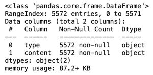

Data Processing

• Removing the unneccesary variables
• Removing null values
• Removing the duplicated values

# Checking missing values
df.isnull().sum()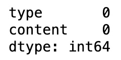

# Removing Null values
df = df.dropna(how='any',axis=0)
row_cnt1 = df.shape[0]
print("The number of rows deleted : %d" % (row_cnt0 - row_cnt1))

The number of rows deleted: 0

There are no missing values in our dataset.

# Checking for the presence of duplicate values. If there exists, we have to remove the rows.
df = df.drop_duplicates()
print("The number of rows removed: %d." % (row_cnt1 - df.shape[0]))

The number of rows removed: 403

There are many dupplicated values.

Visualizing of Data

# Visualizing frequency of target variable
plt.figure(figsize=(8, 6))
ax = sns.countplot(x='type', data=df)
for container in ax.containers:
    ax.bar_label(container)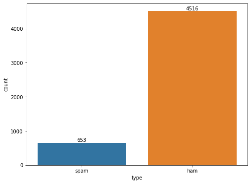

Converting String Variables Into Numerical Variables

All the calculations are performed only with numbers. Thus, we need to convert the useful features into numbers.

There are many methods to convert a corpus to a numerical vector. The simplest approach is the bag-of-words. The bag of words model is a simple document embedding technique based on word frequency. Conceptually, we think of the whole document as a “bag” of words, rather than a sequence. We represent the document simply by the frequency of each word.

First, we have to split a message into its individual words and remove very common words called stopword(‘the’, ‘a’, …). NLTK package allows us to do such works, providing so many useful functions.

import string
import nltk
nltk.download('stopwords')
from nltk.corpus import stopwords

def remove_stopwords(text):
    ### This function is to remove punctuations and stopwords. ###
    
    text = str(text)
    # Removing punctuation
    text = ''.join([letter for letter in text if letter not in string.punctuation])

    # Removing stopword
    stop_word = stopwords.words('english')
    text = ' '.join([item for item in text.split() if item.lower() not in stop_word])
    
    return text

X = df['content'].map(remove_stopwords)
y = df['type']
X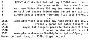

# Saving names of categories in the specific column
encoded_label_names = {}
encoded_label_names['type'] = df['type'].unique()
encoded_label_names

y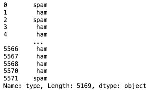

y = y.replace(('ham','spam'),(1,0))
y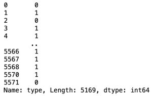

Train-Test Split

# data split
X_train, X_test, y_train, y_test = train_test_split(X, y, train_size = 0.8, test_size = 0.2, random_state = 50)

X_train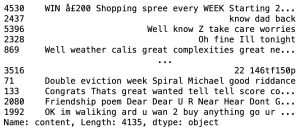

y_train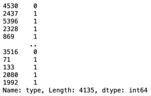

Converting Text Into Numerical Matrix

Bag of Words used to convert words in a text into a matrix representation by extracting its features, it shows us which word occurs in a sentence and its frequency, for use in modeling such as machine learning algorithms.

• Each word occurrence frequency is processed as a feature.
• The vector of all the word frequencies for a given document is considered a multivariate sample.

# import CountVectorizer to convert text into matrix
from sklearn.feature_extraction.text import CountVectorizer

vector = CountVectorizer()
X_train = vector.fit_transform(X_train)

vector.get_feature_names()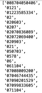

X_train

X_train = pd.DataFrame(X_train.toarray(), columns=vector.get_feature_names())

X_train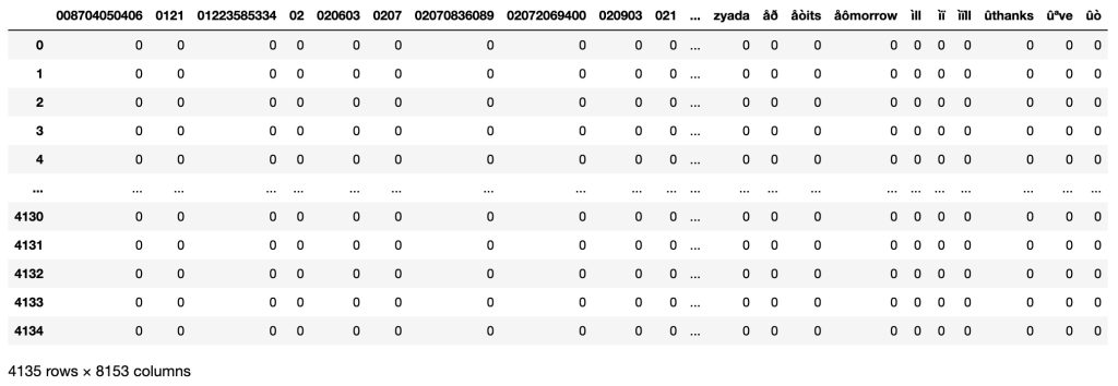

X_train.columns

Building Naive Bayes Classification Model

Because the predictors take up a discrete value, we can use Multinomial naive bayes classifier model.

# Creating instance of model
model = MultinomialNB()

# Fitting train data
model.fit(X_train, y_train)

# Predicting based on train data
y_pred_train = model.predict(X_train)

Now X_test is string variable. To test with X_test, we need to convert X_test into matrix.

# Converting text into matrix
X_test = vector.transform(X_test).toarray()

# Predicting based on test data
y_pred_test = model.predict(X_test)

X_test

Model Evaluation

Comparison of accuracies for train and test datasets.

print('accuracy score for train dataset: %f.3' % accuracy_score(y_train, y_pred_train))
print('accuracy score for test dataset: %f.3' % accuracy_score(y_test, y_pred_test))

accuracy score for train dataset: 0.992261.3
accuracy score for test dataset: 0.986460.3

Confusion Matrix

A confusion matrix is a performance evaluation tool in machine learning, representing the accuracy of a classification model. It displays the number of true positives, true negatives, false positives, and false negatives.

• True positives (TP) occur when the model accurately predicts a positive data point.
• True negatives (TN) occur when the model accurately predicts a negative data point.
• False positives (FP) occur when the model predicts a positive data point incorrectly.
• False negatives (FN) occur when the model mispredicts a negative data point.

# confusion matrix
from sklearn.metrics import confusion_matrix

confusion_m = confusion_matrix(y_test, y_pred_test)

sns.heatmap(confusion_m, annot=True, fmt='d', cmap='YlGnBu_r')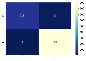

Classification Report

from sklearn.metrics import classification_report

print(classification_report(y_test, y_pred_test))

encoded_label_names

y_pred_test_by_labelname = encoded_label_names['type'][y_pred_test]
y_test_by_labelname = encoded_label_names['type'][y_test]

y_test_comparison = pd.DataFrame(data=zip(y_test_by_labelname, y_pred_test_by_labelname),columns=["original",'predicted'])
y_test_comparison.head(100)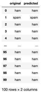

Conclusion

In our task, the accuracy of our model is 98% more and is very high. Therefore, we can use Naive Bayes model to classify if a message sent from a email is spam or ham.